10. Fixed points and linear stability

Lasting Infection and steady-state

Compartmental models like the SIR model are highly flexible. The modeler can add compartments that allow animals to belong to other disease states (e.g. hospitalization, death, subtypes of infection, etc.), and they can model parameters that depend on time or on covariates (e.g. influenza is thought to depend on the specific humidity in the environment).

Lets examine three different types of models and methods to analyze them.

SI model

We’ll start with the SI model. Animals can belong to two disease states: susceptible or infected.

(10.1)\[\begin{align} \frac{dS}{dt} &= -\beta S \frac{I}{N} \\ \frac{dI}{dt} &= \beta S \frac{I}{N} \end{align}\]

From the above system we see that once an animal is infected they will never clear the infection. This is life-long infection. Example of pathogens that infect animals life-long are: HIV, Varicella, and the Herpes virus.

One way to understand the behavior of a model is to estimate the steady-state. For a dynamical system, like compartmental models, the steady state is a vector of values, one for each state, such that if the system starts at those values they remain there forever. A typical method to estimate the steady-state for a system is to find the values (in our case the value of S and I) such that the rate of change is zero.

(10.2)\[\begin{align} \frac{dS}{dt} &= -\beta S \frac{I}{N} = 0 \\ \frac{dI}{dt} &= \beta S \frac{I}{N} = 0 \end{align}\]

The system

(10.3)\[\begin{align} -\beta S \frac{I}{N} &= 0 \\ \beta S \frac{I}{N} &= 0 \end{align}\]

will equal zero when either \(S=0\) (and so then I=N), or if \(I=0\) (and so then \(S=N\)). The first steady state is intuitive. Because an infector is always infectious, over an infinite amount of time every animal will become infected. The second state too is intuitive, if there exist no infector in the population and because no infected animals can enter the system, the population will always remain susceptible. This steady-state is so common that it is given the name Disease Free Equilibirum.

Mathematical aside

Steady states can be repulsive or attracting. To understand the behavior near steady states, we can investigate the behavior of

(10.4)\[\begin{align} x(t) = x^{*} +\epsilon(t). \end{align}\]

for the differential equation

(10.5)\[\begin{align} \frac{dx}{dt} = f(x). \end{align}\]

where \(x^{*}\) are the values of our steady state. That is, we can describe the behavior of solutions a tiny bit away from the steady state. Do they contract back to the steady state? Do they instead move further away?

We can look at the derivative, the rate of change of \(x(t)\) and so \((\epsilon(t))\),

(10.6)\[\begin{align} \frac{dx}{dt} = \frac{ d [ x^{*} + \epsilon(t)]}{dt} = f(x) &= f(x^{*} + \epsilon(t))\\ \frac{ d [ x^{*} + \epsilon(t)]}{dt} &= f(x^{*} + \epsilon(t)) \\ \frac{ d [ \epsilon(t)]}{dt} &= f(x^{*} + \epsilon(t)) \hspace{3mm} (x^{*} \text{ is a constant}) \\ \frac{d \epsilon}{dt} &= f(x^{*}) + \epsilon(t) \left[ f^{'}(x^{*}) \right] \\ \frac{d \epsilon}{dt} &= \epsilon(t) \left[ f^{'}(x^{*}) \right] \\ \epsilon(t) \propto e^{\left[ f^{'}(x^{*}) \right] t} \end{align}\]

This means that if we take the derivative of the right hand side of out differential equation then we can understand if the small perturbations away from the steady state move back to \(x^{*}\), when \(f^{'}(x^{*})<0\) or if small perturbations cause the state to move further away from the steady-state \( f^{'}(x^{*})>0\).

Behavior of SI steady-states

Lets look at the rate of infectors for the SI system, remembering that \(S+I=N\)

(10.7)\[\begin{align} \frac{dI}{dt} &= \beta S \frac{I}{N}\\ &= \frac{\beta I\left( N-I \right)}{N} \end{align}\]

Lets take the Disease Free Equilibrium (I=0) and study the behavior of a small perturbation from this, or \(x(t) = 0 + \epsilon(t)\). This can be read as “My solution will starts at disease free equilibrium plus some small positive value away from this point”.

(10.8)\[\begin{align} \frac{dI}{dt} &= \frac{\beta I\left( N-I \right)}{N}\\ \frac{d[x^{*} + \epsilon(t)]}{dt} &= \frac{\beta (0+\epsilon) \left( N-(0+\epsilon) \right)}{N}\\ \frac{d[x^{*} + \epsilon(t)]}{dt} &= \frac{\beta \epsilon \left( N-\epsilon \right)}{N} \end{align}\]

Lets stop a minute and try to understand

(10.9)\[\begin{align} \frac{d[x^{*} + \epsilon(t)]}{dt} \end{align}\]

We know that our steady state \(x^{*}\) is a constant. We’re asking “What is the rate of change of a constant plus some function \(\epsilon(t)\)?”. Because a constant does not change

(10.10)\[\begin{align} \frac{d[x^{*} + \epsilon(t)]}{dt} = \frac{d\epsilon(t)}{dt} \end{align}\]

Lets look at an example, the line

(10.11)\[\begin{align} \epsilon(t) = 2 + 4 t \end{align}\]

We know that the derivative, the rate of change, for a line is the slope (in this example the value 4). Let \(x^{*} = -10\) and instead ask for the rate of change of

(10.12)\[\begin{align} x^{*} + \epsilon(t) &= -10 + \left(2 + 4 t\right) \\ &= -8 + 4 t. \end{align}\]

When we shift our funciton by a constant the slope does not change—its still four. For this reason, shifting our function by the constant \(x^{*}\) has no effect on the rate of change (i.e. the slope)

(10.13)\[\begin{align} \frac{d[x^{*} + \epsilon(t)]}{dt} = \frac{d\epsilon(t)}{dt}. \end{align}\]

Lets apply this idea to our infectious disease system

(10.14)\[\begin{align} \frac{d[x^{*} + \epsilon(t)]}{dt} &= \frac{\beta \epsilon \left( N-\epsilon \right)}{N}\\ \frac{d\epsilon(t)}{dt} &= \frac{\beta \epsilon \left( N-\epsilon \right)}{N}\\ \end{align}\]

Note, if the rate of change of epsilon is positive then \(\epsilon(t)\) will grow away from the steady state. The steady state will be called repelling. Instead, if the rate of change is negatvie then \(\epsilon(t)\) will shrink towards the stead state. The steady state will be called attracting.

If \(\epsilon\) is a small positive number (say 0.5) then

(10.15)\[\begin{align} \frac{\epsilon(t)}{dt} &= \frac{\beta \times 0.5 \times \left( N-0.5 \right)}{N}, \end{align}\]

and because N is likely greater than 0.5 and \(\beta\) is a positive number, \(\epsilon(t)\) will grow away from the steady-state (called the disease free equilibrium). The disease free equilibrium is a repelling state.

We can use the same reasoning for the \(I=N\) steady state

(10.16)\[\begin{align} \frac{N-\epsilon(t)}{dt} &= \frac{\beta \times (N-1) \times \left( N-(N-1) \right)}{N}\\ \frac{-d \epsilon(t)}{dt} &= \frac{\beta \times (N-1) \times \left( N-(N-1) \right)}{N}\\ \frac{d \epsilon(t)}{dt} &= -\frac{\beta \times (N-1) \times \left( N-(N-1) \right)}{N} \end{align}\]

For the same reasoning, the change in \(\epsilon\) will be negative. The steady state is attracting.

This was a fun mathematical exercise, but what does this mean in the context of public health and outbreaks? If a pathogen is introduced in a population that exhibits SI dynamics, then even a very very small number of infectors will cause the entire population to be infected (DFE is repelling). If, instead, we observe a population with a large proportion of infected individuals that also exhibit SI dynamics then it will be difficult to move them towards a DFE.

Bifurcation analysis to understand the behavior of our system

We know how to compute fixed points and their stability (attracting fixed points vs repelling). However, for many dynamical systems we expect that the value stability of these fixed points to depend on the parameters of our model.

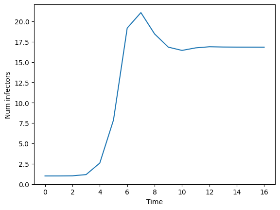
Lets choose as an example the SIRS model

(10.17)\[\begin{align} \frac{dS}{dt} &= -\beta SI/N + \phi R \\ \frac{dI}{dt} &= \beta SI/N - \gamma I \\ \frac{dR}{dt} &= \gamma I - \phi R \end{align}\]

import numpy as np                     #--for array and matrix computations 
from scipy.integrate import solve_ivp  #--needed to solve the ODE system 
import matplotlib.pyplot as plt        #---for plotting 

def sirs(t,y,beta,gamma,phi,n):
    s,i,r = y         #<- We assume that y holds the values s,i,r at each tiny time step from start to end  
    ds_dt = -beta*s*(i/n) + phi*r    
    di_dt =  beta*s*(i/n) - gamma*i
    dr_dt =  gamma*i - phi*r
    return [ds_dt, di_dt, dr_dt] #<-- Its our job to compute the derivatives and return them as a list

beta  = 2
gamma = 1
phi   = 1./2

start,end = 0,30

#--set the number of S,I,R at time 0. 
S0 = 100
I0 = 1
R0 = 0.

#--Compute the total number of individuls (n)
n  = S0+I0+R0 

initial_conditions = (S0,I0,R0) #<--Grouped initial conditions into a tuple


solution = solve_ivp( fun     = sirs
                     , t_span = (start,end)
                     , y0     = initial_conditions
                     , args   = (beta,gamma,phi, n) )

#--Extract solutions from the object called "solution"
times = solution.t
St    = solution.y[0,:] #<-first row  is S
It   = solution.y[1,:] #<-second row is I
Rt   = solution.y[2,:] #<-third row  is R


fig,ax = plt.subplots()

ax.plot(It)
ax.set_xlabel("Time")
ax.set_ylabel("Num infectors")
plt.show()

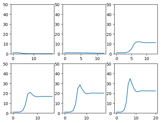
We suspect that different transmission rates will impact the number of infectors long-term. One approach to explore this idea is to plot the number of infectors over time for a finite number of tramission rates.

def compute_SIRS(beta=0):
    
    def sirs(t,y,beta,gamma,phi,n):
        s,i,r = y         #<- We assume that y holds the values s,i,r at each tiny time step from start to end  
        ds_dt = -beta*s*(i/n) + phi*r    
        di_dt =  beta*s*(i/n) - gamma*i
        dr_dt =  gamma*i - phi*r
        return [ds_dt, di_dt, dr_dt] #<-- Its our job to compute the derivatives and return them as a list
    
    gamma = 1
    phi   = 1./2
    
    start,end = 0,30
    
    #--set the number of S,I,R at time 0. 
    S0 = 100
    I0 = 1
    R0 = 0.
    
    #--Compute the total number of individuls (n)
    n  = S0+I0+R0 
    
    initial_conditions = (S0,I0,R0) #<--Grouped initial conditions into a tuple
    
    
    solution = solve_ivp( fun     = sirs
                         , t_span = (start,end)
                         , y0     = initial_conditions
                         , args   = (beta,gamma,phi, n) )
    
    #--Extract solutions from the object called "solution"
    times = solution.t
    St    = solution.y[0,:] #<-first row  is S
    It   = solution.y[1,:] #<-second row is I
    Rt   = solution.y[2,:] #<-third row  is R

    return It

fig , axs = plt.subplots(2,3)
axs = axs.flatten()

list_of_beta_values = [0.5,1.,1.5,2.,2.5,3.]
for ax,beta in zip(axs,list_of_beta_values):
    I = compute_SIRS(beta)
    ax.plot(I)
    ax.set_ylim(0,50)
plt.show()

This is ok, but might be a bit difficult to summarize, especially if there are a lot of plausible transmission rates.

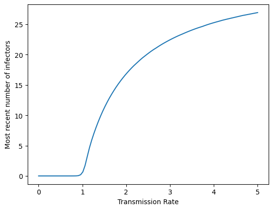
We want to understand the long-term behavior of the number of infectors for different values of the transmission rate \(\beta\). To do this, we might instead decide to run the following algorithm

1. Input a \(\beta\) value

2. Run the SIRS model for many time points

3. Extract the number of infectors at the last time point

4. Plot \(\beta\) against the number of infectors in (3).

This is called a bifurcation diagram. A plot where the horizontal axis varies a parameter (in our example \(\beta\)) and the vertical axis presents a summary statistic (in our example the number of infectors at the most recent time) is called a bifurcation diagram.

betas = np.linspace(0,5,100)

last_vals = []
for beta in betas:
    I = compute_SIRS(beta)
    last_val = I[-1]
    last_vals.append(last_val)

plt.plot(betas,last_vals)
plt.xlabel("Transmission Rate")
plt.ylabel("Most recent number of infectors")
plt.show()

We see, much more clearly, how the behavior of the SIRS model changes as the transmission rate changes. The number of infectors is small and near zero when the transmission rate is below 1. After this, the number of infectors long-term increases similar to the square root of \(\beta\).

Homework

1. Consider the SI model with vital dynamics

(10.18)\[\begin{align} \frac{dS}{dt} &= N \mu - \beta S \frac{I}{N} - \mu S \\ \frac{dI}{dt} &= \beta S \frac{I}{N} - \mu I \end{align}\]

where the term \(N \mu\) represents an influx of susceptibles into the population, and \((- \mu S)\) and (\(- \mu I\)) represent individuals dieing at a rate of \(\mu\) which do not necessarily have to do with the pathogen under study. Please compute the two steady-states for this system. Hint: One if the Disease Free Equilibirum.

2. For the SI model with vital dynamics above, what is the proportion of infected individuals in both steady states? Hint: take a similar approach to this problem as we did the SI model without vital dynamics.

3. Please produce a bifurcation diagram for the SI model with vital dynamics. Lets set \(1/\mu = 70\). For initial conditions, set \(S=100\) and set \(I=1\). That is, we will look primarily at the steady state which is not the disease free equilibirum. Vary the transmission rate from 0 to 2 by increments of 0.1 and plot the transmission rate versus the number of infectors after some long period of time (t=1000 time units is reasonable).

4. In problem (2) you computed two “analytical” steady-states: a disease-free equilibrium and “another” steady-state. For the same tranmission rate values as in problem (3) plot beta versus the analytical solution of your steady-state. One the same plot, overlay the plot produced in (3). Do they match (and why)?