Transformations

Transformations of a random variable

There are times that we may wish to summarize the behavior of a random variable. One common way to describe how probability is distributed among values in the support of a random variable is by computing some function of that random variable.

Discrete random variables

Multiplying and adding a constant to a random variable

Suppose we have defined a random variable \(X\) and wish to study a new random variable \(Y = g(X)\) that is a function of \(X\). The values and the probabilities assigned to \(X\), along with the function \(g\) will determine the values in the support of \(Y\) and assigned probabilities to these values.

Translation

Define a random variable \(X\) with p.m.f. \(f_{X}\) and a new random variable \(Y = X+c\) where \(c\) is a constant. Then the support for \(Y\), \(supp(Y) = \{ x+c | x \in supp(X) \}\) and the p.m.f. of \(Y\), \(f_{Y}(y)\) is

(80)\[\begin{align} f_{Y}(y) &= P(Y=y) \\ &= P(X+c = y)\\ &= P(X=y-c)\\ &= f_{X}(y-c) \end{align}\]

In otherwords, the probability distribution on \(Y\) is \(\mathbb{P} = \{ (y,p) \;|\; y=x+c \text{ and } P(X=x) = p \}\). This type of transformation of the random variable \(X\) to \(Y\) is called a \textbf{translation}.

\ex Suppose we define a random variable \(Z\) such that \(supp(Z) = \{0,1,2,3,4,5\}\) and

(81)\[\begin{align} f_{Z}(z) = \begin{cases} 0.10 & \text{ if } z=0\\ 0.05 & \text{ if } z=1\\ 0.20 & \text{ if } z=2\\ 0.12 & \text{ if } z=3\\ 0.07 & \text{ if } z=4\\ 0.58 & \text{ if } z=5 \end{cases} \end{align}\]

We can define a new random variable \(Y = Z-4\). This random variable will have \(supp(Y) =\{-4,-3,-2,-1,0,1\}\) and

(82)\[\begin{align} f_{Y}(y) = \begin{cases} 0.10 & \text{ if } y=-4\\ 0.05 & \text{ if } y=-3\\ 0.20 & \text{ if } y=-2\\ 0.12 & \text{ if } y=-1\\ 0.07 & \text{ if } y=0\\ 0.58 & \text{ if } y=1 \end{cases} \end{align}\]

Scaling

Define a random variable \(X\) with p.m.f. \(f_{X}\) and a new random variable \(Y = c \cdot X\) where \(c\) is a constant. Then the support for \(Y\), \(supp(Y) = \{ c \cdot x | x \in supp(X) \}\) and the p.m.f. of \(Y\), \(f_{Y}(y)\) is

(83)\[\begin{align} f_{Y}(y) &= P(Y=y) \\ &= P(cX = y)\\ &= P(X=y/c)\\ &= f_{X}(y/c) \end{align}\]

When we multiply or divide a random variable by a constant to produce a new random variable this is called \textbf{scaling}.

\ex Suppose we define a random variable \(Z\) such that \(supp(Z) = \{0,1,2,3,4,5\}\) and

(84)\[\begin{align} f_{Z}(z) = \begin{cases} 0.10 & \text{ if } z=0\\ 0.05 & \text{ if } z=1\\ 0.20 & \text{ if } z=2\\ 0.12 & \text{ if } z=3\\ 0.07 & \text{ if } z=4\\ 0.58 & \text{ if } z=5 \end{cases} \end{align}\]

We can define a new random variable \(Y = 4 \cdot Z\). This random variable will have \(supp(Y) =\{0,4,8,12,16,20\}\) and

(85)\[\begin{align} f_{Y}(y) = \begin{cases} 0.10 & \text{ if } y= 0\\ 0.05 & \text{ if } y= 4\\ 0.20 & \text{ if } y= 8\\ 0.12 & \text{ if } y= 12\\ 0.07 & \text{ if } y= 16\\ 0.58 & \text{ if } y= 20 \end{cases} \end{align}\]

General transformation of a discrete random variable

We explored translation and scaling as specific ways to use one random variable to generate another. However, there are many functions we can apply to a random variable \(X\) to create a new random variable \(Y\), and we need a more general method to compute the probability mass function for \(Y\).

Build a random variable \(X\) and define \(Y\) to be a new random variable such that \(Y = g(X)\). Then the support for \(Y\) is \(supp(Y) = \{y | y = g(x) \text{ and } x \in supp(X) \}\), and

(86)\[\begin{align} f_{Y}(y) = f_{X}(x_{1}) + f_{X}(x_{2}) + \cdots f_{X}(x_{n}) \end{align}\]

where \(x_{1},x_{2}, \cdots x_{n} \in g^{-1}(y)\). If \(Y\) is a function of \(X\) then the probability that the random variable \(Y\) will assign to the value \(y\) is the sum of the probabilities the random variable \(X\) assigns to the set of values \(x_{1},x_{2},\cdots,x_{n}\) that are mapped to \(y\) by the function \(g\).

In more precise mathematical notation, we can say that

(87)\[\begin{align} f_{Y}(y) = \sum_{ x \in g^{-1}(y) } f_{X}(x) \end{align}\]

Example Let \(X\) be the random variable with p.m.f

(88)\[\begin{align} f_{X}(x) = \begin{cases} 0.01 & \text{ if } x=-2 \\ 0.05 & \text{ if } x =-1\\ 0.50 & \text{ if } x=0\\ 0.34 & \text{ if } x=1\\ 0.10 & \text{ if } x=2 \end{cases} \end{align}\]

and also build a new random variable \(Y = X^{2}\). Here the function \(g\) is \(g(x) = x^{2}\). The support of \(Y\) is

(89)\[\begin{align} supp(Y) & = \{ -2^{2},-1^{2},0^{2},1^{2},2^{2} \}\\ & = \{ 4,1,0,1,4 \}\\ & = \{ 0,1,4 \} \end{align}\]

To compute \(P(Y=0)\) we need to sum up the probabilities of all values in \(supp(X)\) that \(g\) maps to \(0\). In our case the only value mapped to \(0\) is the value \(0\), and so \(P(Y=0) = P(X=0) = 0.50\). To compute \(P(Y=1)\) we need to sum the probabilities of all values that \(g\) maps to the value \(1\). In this case two values in \(X\) map to \(1\), the values \(-1\) and \(1\), and so \(P(Y=1) = P(X=-1) + P(X=1) = 0.05+0.34=0.39\). Finally, \(P(Y=4) = P(X=-2) + P(X=2) = 0.11\) (why?). The pm.f for \(Y\) is

(90)\[\begin{align} f_{Y}(y) = \begin{cases} 0.50 & \text{ if } y=0\\ 0.39 & \text{ if } y=1\\ 0.11 & \text{ if } y=4\\ \end{cases} \end{align}\]

Continuous random variables

We can try to follow the same steps for continuous random variables that we followed for discrete random variables. However, we quickly meet a roadblock that must be solved.

Translation

Suppose the random variable \(X\) is a continuous random variable, \(X \sim f\), and that \(Y = X + c\) where \(c\) is a constant.

(91)\[\begin{align} X &\sim f_{X}; supp(X) = [a,b] \\ Y &= X + c \end{align}\]

The first step is to compute the support. To compute the support for \(Y\), we reason the same as when we computed the support for a discrete random variable. That is, we map every value \(x\) in the \(supp(X)\) to to the value \(x+c\). That is,

(92)\[\begin{align} supp(Y) = \{ x+c | x \in supp(X) \} \end{align}\]

In the above case, \(supp(Y) = [a+c, b+c]\)

Next, we can attempt to follow the same steps for computing the probability mass function

(93)\[\begin{align} P(Y=y) &= P(X+c = y) \end{align}\]

but we have a problem. The above is not a probability, or, the probability of any single value for a continuous random variable is zero.

(94)\[\begin{align} P(Y=y) &= P(X+c = y) = 0 \end{align}\]

for all values \(y \in supp(Y)\).

How can we solve this issue? Well for discrete random variables, we expressed the probability of our transformed random variable (\(Y\))in terms of the probability that we assign to (potentially a set) values that map to the value \(y\). Continuous random variables do not assign probability to single values—they assign probabilities to intervals. For continuous random variables, is there a natural choice that we can use to produce a statement similar to

(95)\[\begin{align} P(Y=y) &= P(X+c = y)? \end{align}\]

The cumulative density function \(F(y) = P(Y \leq y)\) assign probabilities to the interval that is all values in the support who are less than the value \(y\). This is a reasonable probability statement that we can use. For continuous random variables, we will work with

(96)\[\begin{align} P(Y \leq y) &= P(X+c \leq y) \end{align}\]

Now we can proceed in exactly the same way as with discrete random variables.

(97)\[\begin{align} P(Y \leq y) &= P(X+c \leq y) \\ &= P(X \leq y - c) \\ &= F_{X}(y-c) \end{align}\]

To compute the probability density function (pdf), we can take the derivative of the above

(98)\[\begin{align} \frac{d F_{x}(y-c)}{dy} &= \frac{d}{dx}F_{X}(y-c) \times \frac{dx}{dy} (y-c) \\ &= f_{X}(y-c) \times 1\\ &= f_{X}(y-c) \end{align}\]

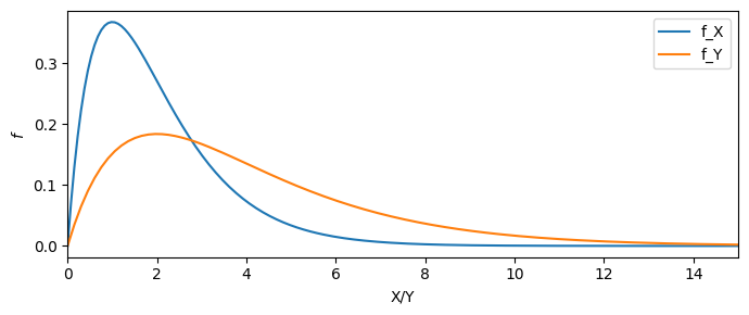
Example Let \(X \sim \text{Exp}(\lambda)\) and \(Y = X + 7\).

(99)\[\begin{align} supp(X) = [0,\infty) \implies supp(Y) = [7, \infty) \\ P(Y \leq y) &= P(X+7 \leq y ) \\ &= P(X \leq y-7) \\ &= F_{X}(y-7) \\ &= f_{X}(y-7) = \lambda e^{ \lambda (y-7) } \end{align}\]

from scipy import stats 


fig,ax=plt.subplots(figsize=(7,3))

domain = np.linspace(0,20,200)
f_x    = stats.expon(scale=2).pdf(domain) 

ax.plot( domain, f_x, label="f_X" )
ax.set_xlim(0,20)
ax.set_xlabel("X/Y")
ax.set_ylabel(r"$f$")

domain = np.linspace(0,20,200)+7
f_y    = stats.expon(scale=2).pdf(domain-7) 

ax.plot( domain, f_y, label="f_Y" )

ax.legend()

fig.set_tight_layout(True)

---------------------------------------------------------------------------
NameError                                 Traceback (most recent call last)
Cell In[1], line 4
      1 from scipy import stats 
----> 4 fig,ax=plt.subplots(figsize=(7,3))
      6 domain = np.linspace(0,20,200)
      7 f_x    = stats.expon(scale=2).pdf(domain) 

NameError: name 'plt' is not defined

Scaling

For scaling, we can take the same approach as with translation.

(100)\[\begin{align} X &\sim f_{X}; supp(X) = [a,b] \\ Y &= cX \end{align}\]

The support is the constant \(c\) times every value in \(supp(X)\) or \(supp(Y) = \{ cx | x \in supp(X) \}\).

The cumulative density function is

(101)\[\begin{align} P(Y \leq y) &= P(cX \leq y) \\ &= P(X \leq y/c) \\ &= F_{X}( y/c ) \\ \end{align}\]

And the probability density can be computed as the derivative of the above

(102)\[\begin{align} f_{Y}(y) &= \frac{d}{dy} F_{X}( y/c ) \\ &= \frac{d}{dx} F_{X}( y/c ) \frac{dx}{dy} (y/c) \\ f_{Y}(y) &= f_{X}(y/c) \frac{1}{c} \end{align}\]

from scipy import stats 

fig,ax=plt.subplots(figsize=(7,3))

domain = np.linspace(0,15,200)
f_x    = stats.gamma(loc=0,a=2,scale=1).pdf(domain) 

ax.plot( domain, f_x, label="f_X" )
ax.set_xlabel("X/Y")
ax.set_ylabel(r"$f$")

domain = np.linspace(0,15,200)*2
f_y    = (stats.gamma(loc=0,a=2,scale=1).pdf(domain/2) )*(1/2)

ax.plot( domain, f_y, label="f_Y" )

ax.set_xlim(0,15)

ax.legend()

fig.set_tight_layout(True)

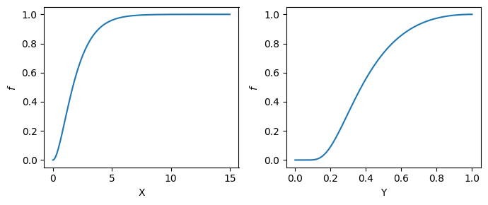
Special case

Lets look at a different type of transformation. Suppose that \(X \sim \text{Exp}(\lambda)\) and that

(103)\[\begin{align} Y = \frac{1}{X+1} \end{align}\]

The support is then

(104)\[\begin{align} supp(X) = [0,\infty) \implies supp(Y) = [0,1) \end{align}\]

What about the probability density? Lets first gain intuition from the cdf.

(105)\[\begin{align} P(Y \leq y) &= P\left(\frac{1}{X+1} \leq y \right) \\ &= P\left( \frac{1}{y} \leq X+1 \right) \\ &= P\left(\frac{1}{y}-1 \leq X \right) = P\left(X \geq \frac{1}{y}-1\right) \end{align}\]

Why did the sign “flip” form less than to greater than or equal to, and how can we right the above in terms of the cdf? Kolmorogov’s axioms. If we divide the support into two intervals (ie two events) \(supp(Y) = [0,y] \cup (y,1] \) then these two events do not intersect. Furthermore, we know that the probability of the support must equal one.

(106)\[\begin{align} P(supp(Y)) &= 1 = P([0,y] \cup (y,1] ) = P([0,y]) + P((y,1]) \\ 1 &= P(Y \leq y) + P(Y>y) \\ P(Y>y) &= 1 - P(Y \leq y) \end{align}\]

Lets apply Kolmogorov’s axioms to our above problem to find that

(107)\[\begin{align} P\left(X \geq \frac{1}{y}-1\right) = 1 - P\left(X \leq \frac{1}{y}-1\right) \end{align}\]

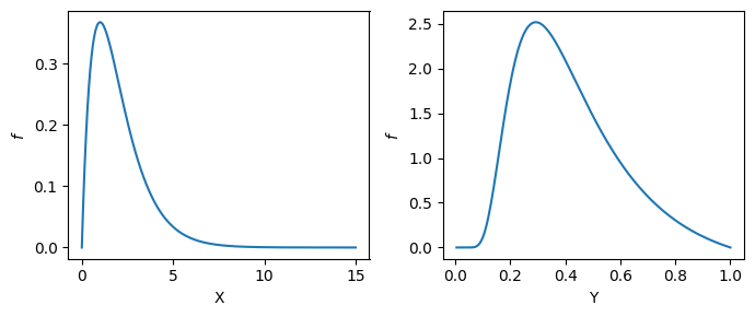
and we can compute the pdf the same as before

(108)\[\begin{align} f_{Y}(y) &= \frac{d}{dx} 1 - P\left(X \leq \frac{1}{y}-1\right) \times \frac{dx}{dy} \frac{1}{y}-1 \\ &= -f_{X}\left(\frac{1}{y}-1\right) \times -\frac{1}{y^{2}}\\ &=f_{X}\left(\frac{1}{y}-1\right) \frac{1}{y^{2}} \end{align}\]

from scipy import stats 

fig,axs=plt.subplots(1,2,figsize=(7,3))

ax=axs[0]
domain = np.linspace(0,15,200)
F_x    = stats.gamma(loc=0,a=2,scale=1).cdf

ax.plot( domain, F_x(domain), label="f_X" )
ax.set_xlabel("X")
ax.set_ylabel(r"$f$")

ax=axs[1]
domain = np.linspace(0,1,200)

ax.plot( domain, 1-F_x( (1./domain)-1), label="f_Y" )
ax.set_xlabel("Y")
ax.set_ylabel(r"$f$")

fig.set_tight_layout(True)

/var/folders/gz/t2mqv3h97_bcfv3l8vcgf5rc0000gp/T/ipykernel_23049/1450322513.py:16: RuntimeWarning: divide by zero encountered in divide
  ax.plot( domain, 1-F_x( (1./domain)-1), label="f_Y" )

from scipy import stats 

fig,axs=plt.subplots(1,2,figsize=(7,3))

ax=axs[0]
domain = np.linspace(0,15,200)
f_x    = stats.gamma(loc=0,a=2,scale=1).pdf

ax.plot( domain, f_x(domain), label="f_X" )
ax.set_xlabel("X")
ax.set_ylabel(r"$f$")

ax=axs[1]
domain = np.linspace(0,1,200)

ax.plot( domain, f_x( (1./domain)-1)/domain**2 , label="f_Y" )
ax.set_xlabel("Y")
ax.set_ylabel(r"$f$")

fig.set_tight_layout(True)

/var/folders/gz/t2mqv3h97_bcfv3l8vcgf5rc0000gp/T/ipykernel_23049/611243278.py:16: RuntimeWarning: divide by zero encountered in divide
  ax.plot( domain, f_x( (1./domain)-1)/domain**2 , label="f_Y" )

(1.0000000000000078, 7.355172166581461e-10)

A general transformation for continuous random variables

If \(g\) is increasing then

(109)\[\begin{align} F_{y} = F_{X}( g^{-1}(y) ) \\ f_{y} = f_{X}( g^{-1}(y) ) \frac{dg^{-1}(y)}{dy} \\ \end{align}\]

(110)\[\begin{align} F_{y} = 1-F_{X}( g^{-1}(y) )\\ f_{y} = -f_{X}( g^{-1}(y) ) \frac{dg^{-1}(y)}{dy} \\ \end{align}\]

Homework

1. Suppose \(X\) is a random variable with support \(supp(X) = \{-2,-1,0,1,2,3\}\) and \(Y = |X|\). Further assume the c.m.f of \(X\) is

   (111)\[\begin{align} F_{X}(x) \begin{cases} 0.05 & \text{ if } x=-2\\ 0.15 & \text{ if } x=-1\\ 0.35 & \text{ if } x=0\\ 0.65 & \text{ if } x=1\\ 0.95 & \text{ if } x=2\\ 1.00 & \text{ if } x=3 \end{cases} \end{align}\]

   1. Define the support of \(Y\)

   2. Build the p.m.f of \(Y\)

   3. Build the c.m.f of \(Y\)

2. The oxygen saturation level (\(S\))of a patient’s blood is used to assess respiratory health. Suppose that due to natural variations and measurement errors, the recorded oxygen saturation (as a proportion between 0 and 1) follows a Beta distribution:

(112)\[\begin{align} S &\sim Beta(\alpha,\beta) \\ f_{S}(s) &= \frac{1}{B(\alpha,\beta)} s^{\alpha-1} (1-s)^{\beta-1} \end{align} \]

Instead of reporting the proportion of Oxygen saturation level, we wish to report the odds. The odds is defined as

(113)\[\begin{align} Y = \frac{S}{1-S} \end{align} \]

Please compute the support and probability density function for \(Y\).

3. In a clinical study, blood pressure deviations from a baseline measurement, \(X\), are assumed to follow a normal distribution due to physiological variations. In some medical analyses, doctors are more interested in the absolute deviation from the baseline

(114)\[\begin{align} Y = |X| \end{align} \]

Please compute the support and probability density function for \(Y\).