Forward problem: (Inversion sampling)

There are many different definitions for what is commonly called “The forward problem”. We will define the forward problem as the following task:

Given a (1) model and (2) parameter values then produce a feasible set of observations

Definition of a model

What do we mean when we say “a model”? A model—in the most abstract terminology—is a collection of probability distributions \(\mathcal{P}\) over a sample space \(\mathcal{G}\) of potential measurements. In other words, we can define a model as the following two objects

(192)\[\begin{align} \mathcal{P} &= \{ F_{\theta} | \theta \in \Theta \}\\ \mathcal{G} &= \{ (x_{1},x_{2}, \cdots, x_{k}) | x_{k} \in \mathbb{R} \} \end{align}\]

where the input for \(F_{\theta}\), the cumulative density function (cdf), is all possible points in the sample space \(\mathcal{G}\). That is, we assume that \(F_{\theta}\) is a cdf that can input points like \((x_{1},x_{2}, \cdots, x_{k})\). Note that every point \(\theta \in \Theta\) will specify exactly one assignment of probabilities to all points in the sample space.

This definition of a model is abstract, but encompasses almost all feasible types of models that we can specify.

Example

Suppose we work for a public health office and are asked to begin modeling the incidence of influenza over during the typical 32-week influenza season. We assume that, for the person requesting this model, it is sufficient to provide a probability density over the potential number of weekly lab-confirmed cases of influenza in the public health office’s jurisdiction. The number of cases that we could observe (could measure) in one week starts at 0 (no cases this week) and end at the total number of individuals living in the jurisdiction (we will call this value \(N\)).

Then the sample space is \(\mathcal{G} = \{ (x_{1},x_{2}, \cdots, x_{32}) \;| \; x_{k} \in [0,N] \}\)

Further, we will assume that the number of cases each week is drawn from a Poisson distribution with parameter \(\lambda\). That is, for week \(k\), we assume \(x_{k} \sim \text{Poisson}(\lambda_{k})\). If we further assume that the number of cases in week \(k\) is statistically independent from cases in week \(l\) then the probability of measuring less than \(x_{k}\) cases in week \(k\) and less than \(x_{l}\) cases in week \(l\) equals

(193)\[\begin{align} F(x_{k},x_{l}) = F(x_{k} | \lambda_{k}) \cdot F(x_{l} | \lambda_{l}) \end{align}\]

where \((\lambda_{k}, \lambda_{l}) \in \mathbb{R}^{+} \times \mathbb{R}^{+}\)

If we can write down our collection of probabilities for two points then we can write this collection for \(32\) points

(194)\[\begin{align} \mathcal{P} = \left\{\prod_{k=1}^{32} F(x_{k} | \lambda_{k}) \;|\; (\lambda_{1},\lambda_{2},\cdots,\lambda_{32} ) \in (\mathbb{R}^{+})^{32} \right\}\\ \end{align}\]

We can generate a dataset—a tuple of possible measurements—from the above model if we are given a set of 32 parameter values and a method for drawing values from the Poisson distribution.

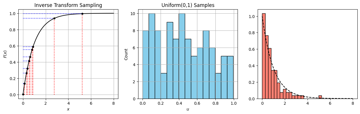
Inverse transform sampling

(195)\[\begin{align} X &\sim f_{X} \\ Y = F_{X}(X) \end{align}\]

(196)\[\begin{align} supp(Y) &= [0,1]\\ \end{align}\]

(197)\[\begin{align}| P(Y < y) &= P( F_{X} < y ) \\ &= P( X < F^{-1}_{X}(y) )\\ &= F_{X}( F^{-1}_{X}(y) ) = y \end{align}\]

(198)\[\begin{align} Y \sim \text{Uniform}(0,1) \end{align}\]

(199)\[\begin{align} Y &\sim \text{Uniform}(0,1) \\ X &= F^{-1}_{X}(Y) \\ \end{align}\]

(200)\[\begin{align} P(X < x) &= P(F^{-1}_{X}(Y) < x) \\ &= P(Y < F_{X}(x) ) \\ &= F_{Y}( F_{X}(x) ) \\ &= F_{X}(x) \end{align}\]

import numpy as np
import matplotlib.pyplot as plt
from scipy.stats import expon

# --- Sampling ---
n_samples = 100
u_samples = np.random.uniform(0, 1, n_samples)
x_samples = -np.log(1 - u_samples)/1  # Inverse CDF of Exp(1)

# For plotting the CDF
x_grid = np.linspace(0, 8, 500)
cdf_vals = expon.cdf(x_grid)

# For highlighting transformation (only show a few)
u_highlight = np.sort(u_samples[:10])
x_highlight = -np.log(1 - u_highlight)

# --- PLOT ---
fig, axs = plt.subplots(1, 3, figsize=(15, 4))

# Plot 1: CDF with inverse transform lines
axs[0].plot(x_grid, cdf_vals, label='CDF of Exp(1)', color='black')
for u, x in zip(u_highlight, x_highlight):
    axs[0].hlines(u, 0, x, color='blue', linestyle='dotted')
    axs[0].vlines(x, 0, u, color='red', linestyle='dotted')
    axs[0].plot(x, u, 'ko', markersize=4)

axs[0].set_title("Inverse Transform Sampling")
axs[0].set_xlabel("$x$")
axs[0].set_ylabel("$F(x)$")
axs[0].grid(True)

# Plot 2: Histogram of uniform(0,1) samples
axs[1].hist(u_samples, bins=15, color="skyblue", edgecolor="black")
axs[1].set_title("Uniform(0,1) Samples")
axs[1].set_xlabel("$u$")
axs[1].set_ylabel("Count")
axs[1].grid(True)

# Plot 3: Histogram of exponential samples
axs[2].hist(x_samples, bins=20, color="salmon", edgecolor="black", density=True, label="Samples")
axs[2].plot(x_grid, expon.pdf(x_grid), 'k--', label='True PDF')  # overlay

[<matplotlib.lines.Line2D at 0x7f2287508d10>]

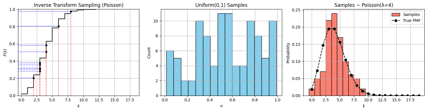
import numpy as np
import matplotlib.pyplot as plt
from scipy.stats import poisson

# Parameters
lam = 4         # Poisson mean
n_samples = 100

# Step 1: Generate uniform samples
u_samples = np.random.uniform(0, 1, n_samples)

# Step 2: Inverse transform sampling for Poisson
def poisson_inverse_transform(u, lam):
    """Perform inverse CDF sampling for Poisson(λ)."""
    k = 0
    cdf = poisson.pmf(k, lam)
    while u > cdf:
        k += 1
        cdf += poisson.pmf(k, lam)
    return k

x_samples = np.array([poisson_inverse_transform(u, lam) for u in u_samples])

# Step 3: CDF grid
k_vals = np.arange(0, 20)
cdf_vals = poisson.cdf(k_vals, lam)

# Use a few points for illustrating transformation
u_highlight = np.sort(u_samples[:10])
x_highlight = [poisson_inverse_transform(u, lam) for u in u_highlight]

# --- Plotting ---
fig, axs = plt.subplots(1, 3, figsize=(15, 4))

# Plot 1: CDF and mapping lines
axs[0].step(k_vals, cdf_vals, where='post', color='black', label='Poisson CDF (λ=4)')

for u, x in zip(u_highlight, x_highlight):
    axs[0].hlines(u, -1, x, color='blue', linestyle='dotted')
    axs[0].vlines(x, 0, u, color='red', linestyle='dotted')
    axs[0].plot(x, u, 'ko', markersize=4)

axs[0].set_xlim(-0.5, max(k_vals))
axs[0].set_ylim(0, 1)
axs[0].set_xlabel('$k$')
axs[0].set_ylabel('$F(k)$')
axs[0].set_title("Inverse Transform Sampling (Poisson)")
axs[0].grid(True)

# Plot 2: Histogram of uniform samples
axs[1].hist(u_samples, bins=15, color="skyblue", edgecolor="black")
axs[1].set_title("Uniform(0,1) Samples")
axs[1].set_xlabel("$u$")
axs[1].set_ylabel("Count")
axs[1].grid(True)

# Plot 3: Histogram of Poisson samples
axs[2].hist(x_samples, bins=np.arange(0, 20) - 0.5, color="salmon", edgecolor="black", density=True, label="Samples")
axs[2].plot(k_vals, poisson.pmf(k_vals, lam), 'ko--', label='True PMF')
axs[2].set_title(f"Samples ~ Poisson(λ={lam})")
axs[2].set_xlabel("$k$")
axs[2].set_ylabel("Probability")
axs[2].legend()
axs[2].grid(True)

plt.tight_layout()
plt.show()

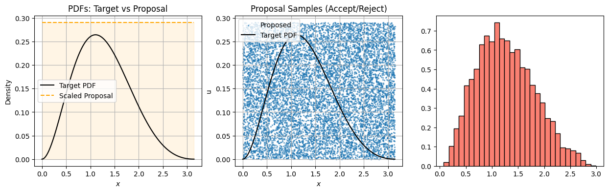
Accept-Reject Sampling: Derivation Using Conditional Densities

We want to simulate from a target distribution ( f(x) ), but we only have access to samples from a proposal distribution ( g(x) ), where:

(201)\[\begin{align} f(x) \leq c \cdot g(x) \quad \text{for all } x \end{align}\]

We define a uniform random variable ( U \sim \text{Uniform}(0, 1) ) and accept the sample ( x \sim g(x) ) if:

(202)\[\begin{align} U < \frac{f(x)}{c g(x)} \end{align}\]

---

Joint Density Over ((x, u))

We define the joint distribution over ( x ) and ( u ):

(203)\[\begin{align} h(x, u) = g(x), \quad \text{for } u \in [0, 1], \; x \in \text{supp}(g) \end{align}\]

The pair ((x, u)) is accepted if:

(204)\[\begin{align} u < \frac{f(x)}{c g(x)} \end{align}\]

---

Step 1: Joint Probability of Acceptance and ( X < x )

We compute the joint probability of ( X < x ) and the sample being accepted:

(205)\[\begin{align} P(X < x, \text{Accept}) &= \int_{-\infty}^{x} \int_{0}^{\frac{f(x)}{c g(x)}} h(x,u) \; du \, dx \\ &= \int_{-\infty}^{x} g(x) \cdot \frac{f(x)}{c g(x)} \; dx \\ &= \frac{1}{c} \int_{-\infty}^{x} f(x) \; dx \end{align}\]

---

Step 2: Marginal Probability of Acceptance

We integrate over the full support:

(206)\[\begin{align} P(\text{Accept}) &= \int_{-\infty}^{\infty} \int_{0}^{\frac{f(x)}{c g(x)}} g(x) \; du \, dx \\ &= \int_{-\infty}^{\infty} g(x) \cdot \frac{f(x)}{c g(x)} \; dx \\ &= \frac{1}{c} \int_{-\infty}^{\infty} f(x) \; dx = \frac{1}{c} \end{align}\]

---

Step 3: Conditional Distribution of ( X \mid \text{Accept} )

Using the definition of conditional probability:

(207)\[\begin{align} P(X < x \mid \text{Accept}) &= \frac{P(X < x, \text{Accept})}{P(\text{Accept})} \\ &= \frac{ \frac{1}{c} \int_{-\infty}^{x} f(x) dx }{ \frac{1}{c} } \\ &= \int_{-\infty}^{x} f(x) dx = F(x) \end{align}\]

Therefore, the accepted samples ( x ) follow the desired distribution ( f(x) )!

---

import numpy as np
import matplotlib.pyplot as plt

# --- Target and Proposal ---
def target_pdf(x):
    return np.exp(-x) * (np.sin(x)**2)  # Not normalized

def proposal_pdf(x):
    return np.ones_like(x)  # Uniform on [0, π]

# --- Settings ---
N = 10000
x_min, x_max = 0, np.pi
x_grid = np.linspace(x_min, x_max, 500)

# Normalize target to get max for rejection
unnormalized = target_pdf(x_grid)
M = 1.1 * np.max(unnormalized)  # Safety buffer
print(f"Using M = {M:.3f} for rejection bound")

# --- Rejection Sampling ---
proposal_samples = np.random.uniform(x_min, x_max, N)
proposal_heights = np.random.uniform(0, M, N)
target_vals = target_pdf(proposal_samples)
accepted = proposal_heights < target_vals

accepted_samples = proposal_samples[accepted]

# --- Plotting ---
fig, axs = plt.subplots(1, 3, figsize=(15, 4))

# Panel 1: Proposal and Target PDFs
axs[0].plot(x_grid, target_pdf(x_grid), label="Target PDF", color='black')
axs[0].plot(x_grid, M * proposal_pdf(x_grid), label="Scaled Proposal", color='orange', linestyle='--')
axs[0].fill_between(x_grid, 0, proposal_pdf(x_grid)*M, color='orange', alpha=0.1)
axs[0].set_title("PDFs: Target vs Proposal")
axs[0].set_xlabel("$x$")
axs[0].set_ylabel("Density")
axs[0].legend()
axs[0].grid(True)

# Panel 2: Proposal samples with rejection
axs[1].scatter(proposal_samples, proposal_heights, s=2, alpha=0.5, label="Proposed")
axs[1].plot(x_grid, target_pdf(x_grid), color='black', label='Target PDF')
axs[1].set_title("Proposal Samples (Accept/Reject)")
axs[1].set_xlabel("$x$")
axs[1].set_ylabel("u")
axs[1].legend()
axs[1].grid(True)

# Panel 3: Accepted Samples
axs[2].hist(accepted_samples, bins=30, density=True, color='salmon', edgecolor='black', label="Accepted Samples")
axs[2].plot(x_grid, target_pdf(x_grid) / np.trapz(target_pdf(x_grid), x_grid), 'k--', label="Target PDF (normalized)")
axs[2].set_title("Accepted Samples ~ Target")
axs[2].set_xlabel("$x$")
axs[2].set_ylabel("Density")
axs[2].legend()
axs[2].grid(True)

plt.tight_layout()
plt.show()

Using M = 0.291 for rejection bound

/tmp/ipykernel_2147/2351102653.py:53: DeprecationWarning: `trapz` is deprecated. Use `trapezoid` instead, or one of the numerical integration functions in `scipy.integrate`.
  axs[2].plot(x_grid, target_pdf(x_grid) / np.trapz(target_pdf(x_grid), x_grid), 'k--', label="Target PDF (normalized)")

Homework

1. [Coding] Code up the Accept/Reject algorithm to sample from the following target distribution \(f_{X}(x) = x^{2}e^{-x}\). We will need to use a proposal distribution \(g(x)\) that is greater than all values for \(f_{X}(x)\). Lets choose as proposal distribution \(g(x) = \lambda e^{-\lambda x}\) with a \(\lambda\) value equal to one.

   1. Present your code

   2. Present a histogram of samples from g

   3. Present a histogram of samples from f (ie accepted samples)

2. In the above example, the distribution \(f_{X}(x)\) is “unnormalized” or the integral over all possible values does not sum to one. This suggests that we can use the Accept/Reject algorithm if we know the unnormalized form of our probability density \(h_{X}(x) = d f_{X}(x)\) for some constant d. Please show using the steps we used previously, that \(P(Y|Accept) = f_{X}(x)\) if

   1. \(Y \sim g(x)\)

   2. \(U \sim \text{Unif}(0,1)\)

   3. Accept a point from y if \(U < \frac{d f_{X}(x)}{c g(x)}\)