
Joint probability#
Two or more random variables#
A single random variable is a useful way to describe a sample space and the probabilities assigned to values on the number line corresponding to outcomes.
But more complicated scientific questions often require several random variables and rules for how they interact. We will explore how to generate multiple random variables on the same sample space. Then we will develop an approach to define probabilities for combinations of random variables, a joint probability mass function and joint cumulative mass function.
A new type of sample space#
Suppose we design a sample space \(\mathcal{S}\) and build two random variables on this space \(X\) and \(Y\). Because \(X\) and \(Y\) are random variables we can think of the support of \(X\) and support of \(Y\) as two new sample spaces. Lets assume that the outcomes in \(supp(X) = \{x_{1},x_{2},x_{3},\cdots,x_{N}\}\) and that the outcomes in \(supp(Y) = \{y_{1},y_{2},\cdots,y_{M}\}\). Then we can define a new set of outcomes in the space \(supp(X) \times supp(Y) = \{x_{i}, y_{j}\}\) for all combinations of \(i\) from \(1\) to \(N\) and \(j\) from \(1\) to \(M\).
This new space above maps outcomes in \(\mathcal{S}\) to a tuple \((x_{i},y_{j})\) where the outcomes were mapped by \(X\) to the value \(x_{i}\) and by \(Y\) to the value \(y_{j}\). If we assign the probability of \((x_{i},y_{j})\) to be the the sum of the probabilities of all outcomes in \(\mathcal{S}\) that \(X\) maps to \(x_{i}\) and \(Y\) maps to \(y_{i}\) then we call this a joint probability distribution.
Example A pharmaceutical company launches a clinical trial to study adverse events from a novel medicine. The trial enrolls patients and randomizes them to receive the novel drug or optimal medical therapy. The trial expects three potential adverse events which we call \(\text{ae}_{1}\), \(\text{ae}_{2}\), and \(\text{ae}_{3}\). We may choose to define a sample space \(\mathcal{S} = \{(\text{nov},\text{ae}_{1}),(\text{nov},\text{ae}_{2}),(\text{nov},\text{ae}_{3}),(\text{omt},\text{ae}_{1}),(\text{omt},\text{ae}_{2}),(\text{omt},\text{ae}_{3})\}\) and further build a random variable \(X\) that maps outcomes to values 0 when an adverse event was experienced by a control patient and 1 when an adverse event was experienced by a novel drug patient, and a random variable \(Y\) that maps adverse event 1 to the value 1, adverse event 2 to the value 2, and adverse event 3 to the value 3.
Event |
X |
|---|---|
(nov, ae₁) |
1 |
(nov, ae₂) |
1 |
(nov, ae₃) |
1 |
(omt, ae₁) |
0 |
(omt, ae₂) |
0 |
(omt, ae₃) |
0 |
Event |
Y |
|---|---|
(nov, ae₁) |
1 |
(nov, ae₂) |
2 |
(nov, ae₃) |
3 |
(omt, ae₁) |
1 |
(omt, ae₂) |
2 |
(omt, ae₃) |
3 |
A joint probability distribution would assign probabilities to all possible pairs of values for \(X\) and \(Y\).
X |
Y |
prob |
|---|---|---|
1 |
1 |
0.10 |
1 |
2 |
0.05 |
1 |
3 |
0.23 |
0 |
1 |
0.05 |
0 |
2 |
0.30 |
0 |
3 |
0.27 |
We write \(P(X=x, Y=y)\) to denote the probability assigned to the joint probability that the random variable \(X\) equals the value \(x\) and the random variable \(Y\) equals the value \(y\). With the above example in mind, \(P(X=0,Y=2) = 0.30\) and this probability could be described as the probability an OMT patient experiences adverse event 2.
Visualization#
Joint probability distributions are often visualized as a table with one random variable’s values representing the rows and the second random variable’s values representing the columns
X \ Y |
Y = 1 |
Y = 2 |
Y = 3 |
|---|---|---|---|
X = 0 |
0.05 |
0.30 |
0.27 |
X = 1 |
0.10 |
0.05 |
0.23 |
Marginal probability#
A joint distribution can be used to compute probabilities that the random variable \(X\) equals the value \(x\) for any value of \(Y\)—\(P(X=x)\) and also the probability that the random variable \(Y\) equals the value \(y\) for any value of \(x\)—\(P(Y=y)\). These probabilities are called marginal probabilities.
Lets assume that our joint probability space over random variables \((X,Y)\) is discrete and can be visualized as
X \ Y |
Y = 1 |
Y = 2 |
Y = 3 |
|---|---|---|---|
X = 0 |
0.05 |
0.30 |
0.27 |
X = 1 |
0.10 |
0.05 |
0.23 |
The marginal probabilities that \(X\) equals \(0\), or \(P(X=0)\), is computed by summing the joint probabilities where \(X=0\). This procedure is, as in the past, the law of total probability. We can apply past procedures to joint probability spaces represetned by several random variables because the rules, laws, and theorems of probability that we learned in chapter one carry over to random variables.
We can use the same procedure to compute the marignal probability that \(X=1\).
The same procedure can be done for the random variable \(Y\) to find marginal probabilities:
Joint probability mass function and cumulative density function#
Let \((X,Y)\) be two random variables defined jointly over the space \(S = supp(X) \times supp(Y)\). Further let random variables \(X\) and \(Y\) be discrete.
Then we define the joint probability mass function as
That is, the joint probability mass function \(f_{(X,Y)}(x,y)\) takes as input an \((x,y)\) and returns the probability of simultaneously observing the values \(x\) and \(y\).
For a pair of continuous random variables, it is more natural to define a joint cumulative density. The joint cumulative density function is defined as
where \( f_{(X,Y)}(x,y)\) is called the joint probability density function. Rather than define each integral over the support, we will assume that a probability density function is defined as zero outside of its support. This allows us to write
** (Numerical) Example** Let \(X\) equal the number of hours until a patient experiences side effects from a medication amd let \(Y\) equal the severity of side effects from that medication. Mild side effects are smaller than more severe side effects. The smallest side effect is zero and the most severe are assigned the value one.
Further, we assume that if a patient quickly experiences a side effect it is because that side effect is mild. This will link X and Y. Small values of \(X\) increase the probability that \(Y\) is near the value zero.
Define the joint pdf as
Then we can plot the probability density for pairs of points between 0 an 5 for \(X\) and between 0 and 1 for \(Y\).
import numpy as np
import matplotlib.pyplot as plt
from matplotlib import cm
from scipy.integrate import dblquad

# Create a grid of x and y values
x = np.linspace(0.01, 5, 200)
y = np.linspace(0.001, 0.999, 200)
X, Y = np.meshgrid(x, y)

# Define the unnormalized joint PDF
def joint_pdf(x, y):
    return y * (1 - y) * np.exp(-x) * np.exp(-5 * y / x)

# Compute the normalizing constant numerically
integral_value, _ = dblquad(joint_pdf, 0.01, 5, lambda x: 0.001, lambda x: 0.999)
C = 1 / integral_value

# Evaluate the normalized joint PDF on the grid
Z = C * Y * (1 - Y) * np.exp(-X) * np.exp(-5 * Y / X)

# Plot the contour
fig, ax = plt.subplots(figsize=(8, 6))
contour = ax.contourf(X, Y, Z, levels=20, cmap=cm.viridis)

# Labels and color bar
ax.set_title('Contour Plot of Joint PDF')
ax.set_xlabel('X (Time until side effects)')
ax.set_ylabel('Y (Severity)')
plt.colorbar(contour, label='f(X, Y)')

plt.tight_layout()
plt.show()
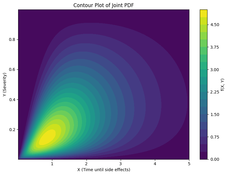
We can see that higher density values tend to appear near where \(X=1\) and \(Y=0.2\)
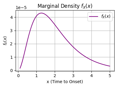
We can use the law of total probability to compute marginal probabilities for continuous variables as well. For our example above,
In our case above, the integral \(\int_{y=0}^{y=1} y (1 - y) e^{-5y/x} \; dy\) , doesnt have an anti-derivative. Instead, we can estimate the integral numerically and recognize that this integral over all y values depends on \(x\). In otherwords
import numpy as np
import matplotlib.pyplot as plt
from scipy.integrate import quad

# Define the integrand for marginal f_X
def integrand(y, x):
    return y * (1 - y) * np.exp(-5 * y / x)

# Define the marginal f_X(x)
def f_X(x):
    integral, _ = quad(integrand, 0, 1, args=(x,))
    return (1 / 219) * np.exp(-x) * integral

# Evaluate over a range of x
x_vals = np.linspace(0.1, 5, 200)
f_x_vals = np.array([f_X(x) for x in x_vals])

# Plot the marginal f_X(x)
plt.figure(figsize=(4, 3))
plt.plot(x_vals, f_x_vals, label=r'$f_X(x)$', color='purple')
plt.title('Marginal Density $f_X(x)$')
plt.xlabel('x (Time to Onset)')
plt.ylabel(r'$f_X(x)$')
plt.grid(True)
plt.legend()
plt.tight_layout()
plt.show()
(Analytical) Example
To complement the above computational example, we present below an exercise that has a closed form solution for the marginal probability over X.
Define the joint pdf over \((X,Y)\) as
We can see that \(X\) depends on the value of \(Y\) because x values must be less than y values.
We can compute the marginal \(f_{X}\) as
Conditional probability#
Given two random variables, X and Y, the conditional probability of the random variable X given a value for the random variable \(Y\) is defined as
This definition is analogous the our previous definition of conditional probability defined over events. We can confirm that \(f_{X|Y}(x,y)\) is indeed a valid probability distribution. Because \(f_{X|Y}(x,y) = \frac{ f_{XY}(X,Y) }{f_{Y}(y)}\) is a result of the division of two probability densities then we know that \(f_{X|Y}(x,y) \ge 0\). Further, we can compute the integral over all values in the support of \(X\) to find
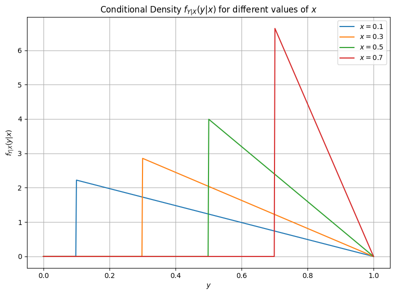
(Analytical) Example Continued
Starting from our above example, lets compute \(f_{Y|X}\). This is then
import numpy as np
import matplotlib.pyplot as plt

# Define the conditional density f_{Y|X}(y|x)
def f_Y_given_X(y, x):
    norm_const = 1 - 2*x + x**2
    return np.where((y > x) & (y < 1), 2*(1 - y) / norm_const, 0)

# Values for x to condition on
x_vals = [0.1, 0.3, 0.5, 0.7]

# Create a fine grid for y
y = np.linspace(0, 1, 500)

# Plot
plt.figure(figsize=(8, 6))
for x in x_vals:
    plt.plot(y, f_Y_given_X(y, x), label=f'$x = {x}$')

plt.title('Conditional Density $f_{Y|X}(y|x)$ for different values of $x$')
plt.xlabel('$y$')
plt.ylabel('$f_{Y|X}(y|x)$')
plt.legend()
plt.grid(True)
plt.tight_layout()
plt.show()
Transformations#
More than two variables#
Joint distributions need not be restricted to only two random variables. We can build joint distributions of any number of random variables and can compute marginal probabilities in the same way that we do for a joint distribution of two random variables.
This is because we can consider a new sample space of values that our random variable can take. Suppose we build two random variables \(X\) that maps outcomes to the the values -1,0,1 and \(Y\) that maps outcomes to the values 1,2,3. We can define a new sample space \(\mathcal{S} = \{(x,y) | x \in supp(X) \text{ and } y \in supp(Y) \}\) With our new sample space, we can now discuss statements like \(P(X = x | Y = y)\).
Example If we continue with our pharmaceutical example, we can build a new sample space \(\mathcal{S} = \{(0,1),(0,2),(0,3),(1,1),(1,2),(1,3)\}\) and compute, for example, \(P(X=1 | Y=2) = \frac{P(X=1,Y=2)}{P(Y=2)} = \frac{0.05}{0.35} = 0.14\).
We can define the conditional probability of the value of one random variable given another as
and so define statistical independence between two random variables, \(A\) and \(B\), as
We can also translate the law of total probability from events to random variables. For a partition \([Y=y_{1}] \cup [Y=y_{2}] \cup [Y=y_{3}] \cup \cdots \cup [Y=y_{n}]\) of the event that the random variable \(X=x\),
By thinking of the values of a random variable as outcomes in a new sample space, we can apply our past intuition and the past mechanics of events, sets to a collection of random variables.
import numpy as np
import matplotlib.pyplot as plt
# Define the PDF
def f(x, y):
return 4 * x * y * np.exp(-(x**2 + y**2))
# Create a grid over [0, 3] x [0, 3]
x = np.linspace(0, 3, 300)
y = np.linspace(0, 3, 300)
X, Y = np.meshgrid(x, y)
Z = f(X, Y)
# Plot
fig = plt.figure(figsize=(10, 6))
ax = fig.add_subplot(111, projection='3d')
ax.plot_surface(X, Y, Z, cmap="viridis", edgecolor='none')
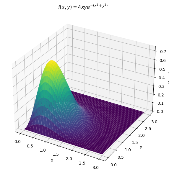
ax.set_title(r"$f(x, y) = 4xy e^{-(x^2 + y^2)}$")
ax.set_xlabel("x")
ax.set_ylabel("y")
ax.set_zlabel("f(x, y)")
plt.tight_layout()
plt.show()
import numpy as np
import plotly.graph_objects as go
import plotly.io as pio

# Use a compatible renderer
pio.renderers.default = "notebook"  # Try "iframe" or "notebook_connected" if needed

# Define the PDF
def f(x, y):
    return 4 * x * y * np.exp(-(x**2 + y**2))

# Grid
x = np.linspace(0, 3, 150)
y = np.linspace(0, 3, 150)
X, Y = np.meshgrid(x, y)
Z = f(X, Y)

# Plot
fig = go.Figure(data=[go.Surface(z=Z, x=X, y=Y, colorscale='Viridis')])
fig.update_layout(
    title=r"$f(x, y) = 4xy e^{-(x^2 + y^2)}$",
    scene=dict(xaxis_title='x', yaxis_title='y', zaxis_title='f(x, y)')
)
fig.show()
---------------------------------------------------------------------------
ModuleNotFoundError                       Traceback (most recent call last)
Cell In[5], line 2
      1 import numpy as np
----> 2 import plotly.graph_objects as go
      3 import plotly.io as pio
      4
      5 # Use a compatible renderer

ModuleNotFoundError: No module named 'plotly'
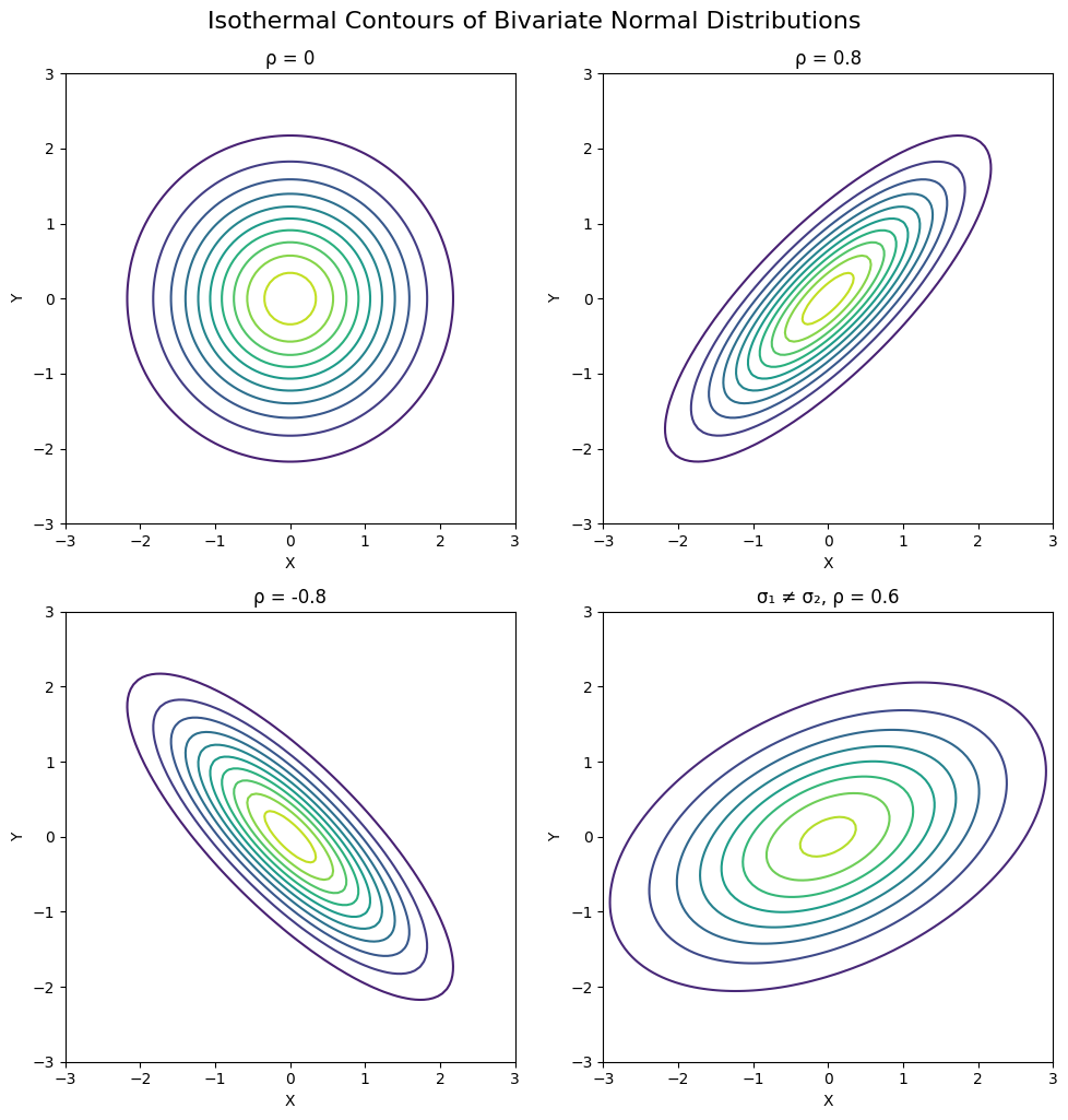
import numpy as np
import matplotlib.pyplot as plt
from scipy.stats import multivariate_normal

# Grid for all plots
x = np.linspace(-3, 3, 100)
y = np.linspace(-3, 3, 100)
X, Y = np.meshgrid(x, y)
pos = np.dstack((X, Y))

# Covariance configurations to compare
covariances = [
    ([[1, 0], [0, 1]], "ρ = 0"),
    ([[1, 0.8], [0.8, 1]], "ρ = 0.8"),
    ([[1, -0.8], [-0.8, 1]], "ρ = -0.8"),
    ([[2, 0.6], [0.6, 1]], "σ₁ ≠ σ₂, ρ = 0.6")
]

# Create 2x2 subplot
fig, axes = plt.subplots(2, 2, figsize=(10, 10))

for ax, (cov, title) in zip(axes.flat, covariances):
    rv = multivariate_normal([0, 0], cov)
    Z = rv.pdf(pos)

    ax.contour(X, Y, Z, levels=10, cmap='viridis')
    ax.set_title(title)
    ax.set_xlabel('X')
    ax.set_ylabel('Y')
    ax.set_aspect('equal')

plt.tight_layout()
plt.suptitle("Isothermal Contours of Bivariate Normal Distributions", fontsize=16, y=1.02)
plt.show()
Exercises#
Define the following joint distribution of random variable \(Q\) and \(R\) that are mapped from the sample space \(\mathcal{G}\)
Q
R
prob
2
1
0.01
2
2
0.075
2
3
0.13
1
1
0.1
1
2
0.05
1
3
0.17
0
1
0.05
0
2
0.30
0
3
0.115
What is the implied support of \(Q\)?
What is the implied support of \(R\)?
Compute P(Q=1,R=2)
Compute the marginal probabilities for \(Q\)
Compute the marginal probabilities for \(R\)
Compute \(P(R=1 | Q=0)\)
The random variable \(Q\) is called statistically independent from \(R\) if for every value \(q \in supp(Q)\) and for every value \(r \in R\) the following is true \(P(Q=q |R=r) = P(Q)\). Is \(Q\) statistically independent from \(R\)? Why or why not?
For two events \(A\) and \(B\) that are statistically independent, we found that \(P(A \cap B) = P(A)P(B)\). Please derive an equivalent expression for two random variables by applying the definition of conditional probability and statistical independence to random variables.
Define the following joint distribution of random variable \(Q\) and \(R\) that are mapped from the sample space \(\mathcal{G}\)
Q
R
prob
2
1
0.01
2
2
0.075
2
3
0.13
1
1
0.1
1
2
0.05
1
3
0.17
0
1
0.05
0
2
0.30
0
3
0.115
Please compute \(\mathbb{E}(Q)\)
Please compute \(\mathbb{E}(R)\)
Please compute \(V(Q)\)
Please compute \(V(R)\)
Kimberly Palaguachi-Lopez—-Class of 2024: Consider the following joint distribution of random variable Z and L that are mapped from the sample space G
Z
L
prob
1
0
0.05
2
0
0.15
3
0
0.19
2
1
0.02
1
1
0.12
3
1
0.04
2
0.5
0.10
3
0.5
0.13
1
0.5
0.20
Please compute the \(supp(Z)\)?
Please compute the \(supp(L)\)?
Solve for \(P(Z=1,L=1)\)
Solve for the respective marginal probabilities of \(Z\)
Solve for the respective marginal probabilities of \(L\)
Is the probability distribution for the random variable Z a valid probability distribution? Why or why not? Is the probability distribution for L a valid probability distribution? Why or why not?
During flu season, a health clinic tracks whether patients report fever (F) and/or cough (C). Based on past data, the joint probabilities of symptoms for a randomly selected patient are given by:
Cough = Yes |
Cough = No |
|
|---|---|---|
Fever = Yes |
0.30 |
0.15 |
Fever = No |
0.25 |
0.30 |
Let ( F ) and ( C ) be binary random variables indicating the presence (Yes) or absence (No) of fever and cough, respectively.
1. **(Joint probability)**
   What is the probability that a patient has both fever and cough?

2. **(Marginal probability)**
   What is the probability that a patient has a cough?

3. **(Conditional probability)**
   Given that a patient has a cough, what is the probability they also have a fever?

4. **(Independence)**
   Are the symptoms fever and cough independent? Justify your answer using the definition of independence in terms of joint and marginal probabilities.

5. **(Interpretation)**
   Briefly explain what your answer to part (4) means in a real-world clinical context.
Suppose that the joint probability density function of systolic blood pressure ( X ) and cholesterol level ( Y ) (in suitable units) in a patient population is modeled by:
1. **(Marginal density)**
   Derive the marginal density $f_X(x) $.

2. **(Conditional density)**
   Compute the conditional density $ f_{Y|X}(y|x) $.

3. **(Validation)**
   Show that your expression for \( f_{Y|X}(y|x) \) is a valid density by integrating over the appropriate support.