The law of large numbers - Plots and Probability

The intuition behind the law of large numbers can be characterized by the fol- lowing experiment: you are asked to flip a fair coin and record the whether the coin is heads up or tails up. After 10 flips you are asked to compute the proportion of heads up flips, after 50 flips you are asked to compute this pro- portion, after 100, 1,000, 10,000 flips you are asked to compute the proportion of heads up flips. We expect that if this coin is fair that the proportion of flips with heads face up will get closer and closer to 0.50.

import matplotlib.pyplot as plt 
import numpy as np

flips = np.arange(1,1000+1)

avg_flips = []
for nflip in flips:
    observations = []
    for flip in range(nflip):
        if np.random.random() < 0.50:
            observations.append(1)
        else:
            observations.append(0)
    mean_of_flips = np.mean(observations)
    avg_flips.append( mean_of_flips )

plt.plot(flips, avg_flips)
plt.xlabel("Number of Flips")
plt.ylabel("Proportion of Heads (represented as a one)");

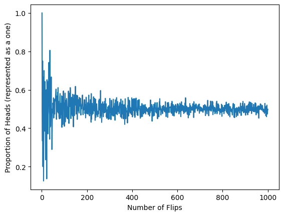
Define a sequence of random variables $X_{1}, X_{2}, \cdots, X_{n}$ such that any pair of random variables, $X_{i}$ and $X_{j}$ are independent (that is $P(X_{i} = x | X_{j} = y) =P(X_{i} = x)$ . Finally, transform this sequence into a single random variable $\overline{X}$ that is equal to $\overline{X} = \dfrac{X_{1} + X_{2} + X_{3} + \cdots X_{N}}{N}$ .

Then the law of large numbers (LLN) states that given any small number $\epsilon$ that is greater than 0 as $n$ grows towards infinity $(n \to \infty)$

\begin{align} P( | \overline{X}_{n} - \mu | > \epsilon ) \to 0 \end{align}

(1)

where $\mu = \mathbb{E}(\overline{X})$ .

We can picture a distribution $Z_{n} = | \overline{X}_{n} - \mu |$ that depends on $n$ and as $n$ increase the random variable $Z_{n}$ assigns more and more probability to the value 0.

Below we show this process and associated random variable $Z_{n}$ for a Bernoulli distributed random variable. The random variable $Z_{n} = \sum_{i=1}^{n} X_{n}/n$ where $X_{n} \sim \text{Bernoulli}(1/2)$ . To estimate the probability density function for $Z_{n}$ , we simulated 400 draws from $Z_{n}$ by drawing a 1 or 0 from $n$ Bernoulli-distributed random variables, taking the average, and appending this to a list. This process of drawing $n$ Bernoulli random variables, computing the average, and appending is repeated 400 times.

num_mean_observs = 400

avg_flips_10 = []
for _ in range(num_mean_observs):
    observations = []
    for flip in range(10):
        if np.random.random() < 0.50:
            observations.append(1)
        else:
            observations.append(0)
        mean_of_flips = np.mean(observations)
    avg_flips_10.append( mean_of_flips )

avg_flips_50 = []
for _ in range(num_mean_observs):
    observations = []
    for flip in range(50):
        if np.random.random() < 0.50:
            observations.append(1)
        else:
            observations.append(0)
        mean_of_flips = np.mean(observations)
    avg_flips_50.append( mean_of_flips )

avg_flips_100 = []
for _ in range(num_mean_observs):
    observations = []
    for flip in range(100):
        if np.random.random() < 0.50:
            observations.append(1)
        else:
            observations.append(0)
        mean_of_flips = np.mean(observations)
    avg_flips_100.append( mean_of_flips )

avg_flips_500 = []
for _ in range(num_mean_observs):
    observations = []
    for flip in range(500):
        if np.random.random() < 0.50:
            observations.append(1)
        else:
            observations.append(0)
        mean_of_flips = np.mean(observations)
    avg_flips_500.append( mean_of_flips )

fig,axs = plt.subplots(1,4, figsize=(9,4))

axs[0].hist(avg_flips_10)
axs[0].set_xlim(0.2,0.8)
axs[0].set_xlabel("Prop of heads")
axs[0].set_ylabel("Frequency")
axs[0].set_title(r"$Z_{10}$")


axs[1].hist(avg_flips_50)
axs[1].set_xlim(0.2,0.8)
axs[1].set_xlabel("Prop of heads")
axs[1].set_ylabel("Frequency")
axs[1].set_title(r"$Z_{50}$")


axs[2].hist(avg_flips_100)
axs[2].set_xlim(0.2,0.8)
axs[2].set_xlabel("Prop of heads")
axs[2].set_ylabel("Frequency")
axs[2].set_title(r"$Z_{100}$")


axs[3].hist(avg_flips_500)
axs[3].set_xlim(0.2,0.8)
axs[3].set_xlabel("Prop of heads")
axs[3].set_ylabel("Frequency")
axs[3].set_title(r"$Z_{500}$")

plt.show()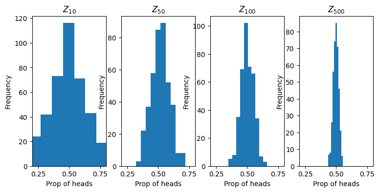

# Homework