Exploratory Data analysis - Plots and Probability

The real work of an expedition begins when you return.--Louise Arner Boyd

Exploratory vs Confirmatory data analysis¶

Exploratory data analysis (EDA) is the study of: the potential for data to answer hypotheses and how to generate novel hypotheses by the study of relationships between collected information. This is in contrast to confirmatory data analysis. Confirmatory data analysis techniques are hypothesis tests, confidence intervals, statistical estimators---methods by which we seek to understand all possible experiments by observing a smaller number of experiments.

Both analyses are important. We will start with EDA.

Descriptive Statistics¶

The goal of descriptive statistics are to characterize a larger set of observations with a smaller set of numbers.

Consider storing the each observation from a set of experiments as a component of a vector.

\begin{align} v = [ v_{1},v_{2},\cdots,v_{N}]^{T} \end{align}

(1)

Its easiest to think of a vector as an ordered list of numbers, in this case our observation.

Then a descriptive statistic is a function ( $f$ ) from $v$ to $\mathcal{R}$ that “best” describes some attribute of this vector or

\begin{align} f: v \to \mathcal{R} \end{align}

(2)

The symbol $\mathcal{R}$ here is called “The Real Line” and includes all positive and negative numbers, including decimals.

Descriptive statistics can help us quickly understand our the data that we have collected and what we can do with this data. The con to using descriptive stats is that because we are using just a few numebrs to represent many there is some loss of information.

Measures of Central Tendancy¶

Before we attempt (and i mean it) to define a measure of central tendancy, its import first to define what we mean by a measure. For this class, a measure is a function that inputs an observation from an experiment and outputs a number on the real line. This is what we often mean we say that we are quantifying something about our experiment. Consider one attribute of an observation, then you can think of mapping every possible characteristic of that attribute you may observe to a numerical value. This is measurement.

Given that you have prescribed a measure for your sample of data and applied it to each observation, then a measure of central tendency aims to use a single value to describe the location by which observations are most typical found.

We will look at two frequent measures of central tendancy, the mean and the median.

But first, lets set the stage with a study. To illustrate the measures of central tendancy, we will use the open source dataset from the study titled Trends in crowd accidents based on an analysis of press reports. A link to the study is here.

In the article abstract, the authors write
Crowd accidents – defined as situations where mass gatherings of people lead to deaths or injuries – have become a frequent occurrence on a global scale. Given the recurring nature of these accidents, it is essential that their characteristics are analyzed. To this end, an important step would be documenting these records. Here, a database of crowd accidents is developed for the period of 1900–2019 through a comprehensive investigation of the press and media reports.

We will use python to take a look at this dataset, which is presented just below.

import pandas as pd 
d = pd.read_csv("https://zenodo.org/records/7523480/files/accident_data_numeric.csv?download=1")
d.head()

Loading...

Every row in the dataset describes a crowd accident collected by the researchers. The columns describe different types of information from each observed crowd accident.

To get a feel for our dataset, we may wish to better understand the sizes of the crowds studied, the number of injured, and the number of fatalities. Two measures of central tendancy that are to give us a sense of where on the measurement scale these observations lie are the mean and median.

The mean and median¶

Given observations $d = [d_{1},d_{2},d_{3},...,d_{n}]$ ,

The mean> is computed as

\begin{align} \bar{d} = (d_{1} + d_{2} + \cdots + d_{n}) / n = \sum_{i=1}^{N} d_{i} / n \end{align}

(3)

Most everyone has experience computing the mean of a dataset. However, if you stop to think about the above algorithm. At its face, it is unusual to think that this produces a summary measure that describes where observations typically fall on a measurement scale. Why does the mean do a good job at summarizing the location?

The mean as most often One explanation is that the mean computes a weighted sum where every measured value is weighted by how frequently it is observed.

Consider the following dataset of measured observations:

\begin{align} \mathcal{D} = (1,2,3,5,3,2,1,7,4,1,7,7,1,2) \end{align}

(4)

using the above formula for the mean, we would compute

\begin{align} \bar{d} = \frac{1+2+3+5+3+2+1+7+4+1+7+7+1+2}{14} \end{align}

(5)

but addition is commutative. We can arrange the above sum in the numerator however we like without changing its total. That is, we would arrive at the same sum if we moved all the same values next to another.

\begin{align} \bar{d} &= \frac{1+1+1+1 + 2+2+2 + 3+3 + 4 + 5 + 7 + 7 + 7}{14} \end{align}

(6)

Now by definition the sum $1+1+1+1$ equals $(4) 1$ and the sum $2+2+2$ equals $(3) 2$ and so on. The the above sum can be simplified, using multiplication, as the frequency that each number appears times its value or

\begin{align} \bar{d} &= \frac{ 4 \cdot 1 + 3 \cdot 2 + 2 \cdot 3 + 1 \cdot 4 + 1 \cdot 5 + 3 \cdot 7 }{14} \end{align}

(7)

Last, but not least, we can distribute the denominator to find that

\begin{align} \bar{d} &= \left(\frac{4}{14}\right) 1 + \left(\frac{3}{14}\right) 2 + \left(\frac{2}{14}\right) 3 + \left(\frac{1}{14}\right) 4 + \left(\frac{1}{14}\right) 5 + \left(\frac{3}{14}\right) 7 \\ \end{align}

(8)

The values in the parentheses are equal to the proportion of times each value is observed in our sample. This is the reason that the mean is a measure of central tendancy. The intuition is that this value called the mean will move closest to the most frequently occuring value in your sample. By doing so, the mean summarizes the typical “location” on the measurement scale for where your data lie.

Given the same set of observations, the median is computed as the middle most value if the number of data points you collected is odd and the mean of the two most middle values if the number of data points you collected is even. The intuition for the median is that a best location for where the data is located is the middle most value (sometimes referred to as the deepest value, see John Tukey’s work).

Lets apply what we learned to the crowd accident dataset by computing the mean and median crowd size, number of injured, and number of fatalities.

Attribute	Mean	Median
Crowd size	X	X
Num. Injured	X	X
Num. Fatalities	X	X

Measures of dispersion¶

Now that we have a handle on summary quantities that describe the typical location of where our data land, we can discuss how variable, spread out, or the typical data “scale” (sequence of ordered marks by which we measure values observed in our data).

Measures of dispersion are meant to capture how observations in a dataset are either close, or far, from one another. A set of observations that are spaced far apart from one another is said to be highly dispersed. Vice versa, data has low dispersion if they are closely grouped together.

Range, Variance, and Standard deviation¶

A common measure of dispersion is the range accompanied by the min and max values. Given a dataset, $\mathcal{D} = (d_{1},d_{2},\cdots,d_{n})$ , the max is the largest observation, the min is the smallest observation, and the range equals the max minus the min.

The min, max, and range are very natural measures of the “stretched out” and “squished togther” property of a measure of dispersion. But, these summary values don’t really tell the scientist a natural marking by which we should measure values to determine if new, incoming observations are quite large, small, or expected.

For this, we will look the variance and standard deviation.

The variance is computed as

\begin{align} v( [d_{1}, d_{2}, \cdots, d_{n}] ) = \sum_{i=1}^{n} \frac{(d_{i} - \bar{d})^{2}}{n} \end{align}

(9)

Why, intuitively, does the variance capture dispersion? The variance could be understood by mapping each data point to a distance from the mean and then computing the average distance. In other words, we can measure the distnace of a data point $d_{i}$ from the mean by applying the function $f(d) = \left( d - \bar{d} \right)^{2}$ to each data point $d_{i}$ . Note, because this quantity is squared it does not matter if $d_{i}$ is smaller/below or larger/above the mean. After we compute these “distances” then take their mean to describe the typical distance from the mean.

Lets look at a short example of comparing the min, max, range, and variance between the counts of two pathogens. We’ll find that the number of cases is a bit more uncertain than the other and consider a natural way to “mark our ruler” for counting cases of a pathogen.

Measles

Measles is a highly contagious, vaccine-preventable viral disease. In the United States, confirmed measles cases are reported to the CDC through the National Notifiable Diseases Surveillance System (NNDSS).

Influenza

Influenza is a vaccine-preventable respiratory infection that exhibits strong seasonal variation. For influenza, we will use the weekly number of influenza-positive specimens reported by U.S. clinical laboratories to the CDC as our measure of influenza activity.

The mean weekly number of reported measles cases over the past year in the United States is XX, while the mean weekly number of influenza-positive specimens is YY. The variance is XX for measles and YY for influenza.

Because the variance of influenza is larger than the variance of measles, influenza observations are more widely dispersed around their mean. In this sense, the mean alone does a poorer job of characterizing a typical week of influenza activity than it does a typical week of measles activity.

That said, the variance has a bit of a problem: the units. For our above examples, the units are measured in “number of cases (we’ll call this cases for simplicity)”.

If out dataset $\mathcal{D} = [d_{1}, d_{2}, \cdots, d_{n}]$ is measured in cases then what are the units for the mean?

To compute the units of an algebraic expression there is a short list of rules. Consider two quantities with units $u$ and $v$ . For example, $u$ might be in units “centimeters” and $v$ in “lbs”.

Rules

You cannot add or subtract two quantities with different units. ( “centimeters” + “lbs” doesnt work. )
When you add/subtract two quantities wit hthe same units then the sum/difference is in the same units. (“centimeters” plus “centimeters” is in “centimeters”)
You cna always multiply/divide two quantities. (“centimeters” times “lbs” is fine.)
When you multiply/divide by two quantities with units u and v then the product has units $u v$ . (“centimeters” times “lbs” is in the units “centimeter lbs”)

Well the mean is computed as

\begin{align} \bar{d} &= \frac{1}{n}\sum_{i=1}^{n} d_{i}\\ \bar{d}_{\text{units}}& = \frac{1}{n}\sum_{i=1}^{n} \text{cases}\\ &= \text{cases} + \text{cases} + \text{cases} + ... \\ &=\text{cases} \end{align}

(10)

In other words, we add together all the values and divide by the (unit-less) (n)umber of datapoints. When we add two quantities that are both in the units “cases” then the same units are return. The mean is in the same units that we used to measure individual data points.

What about the variance? Lets just look at how we compute the variance for two data points.

$var(\mathcal{D}) = \frac{1}{2}( d_{1} - \bar{d} )^{2} + ( d_{2} - \bar{d} )^{2}$ .

Lets look at what happens to units.

\begin{align} var_{\text{units}}(\mathcal{D}) &= \frac{1}{2}( \text{cases} - \text{cases} )^{2} + ( \text{cases} - \text{cases} )^{2} \\ &= \frac{1}{2}( \text{cases} )^{2} + ( \text{cases} )^{2} \\ &= ( \text{cases} )^{2} \end{align}

(11)

If our datapoints are measured in cases then variance is measured in cases squared. What the heck is cases squared. There is not a readily avalable intuitive description of squared units for many measurement systems.

To move the variance back into our original units we need to get rid of that squared term. Lets just take the square root.

The standard deviation (sd) is defined as the square root of the variance or $\text{sd}(\mathcal{D}) = \left(\text{var}(\mathcal{D})\right)^{1/2}$ . Importantly, if your data points are measured in units $u$ then the standard deviation is also measured in units $u$ ---the same units.

An intrinsic measurement system¶

In only a few applications do we know a good measurement system. One that allows us to discuss units of a quantitiy with precision and one where a unit has a meaningful different in some represented phenomena. However, in many applciations we dont have a good sense of the measurement system we should use before (or really after too) collecting the data.

For example, we may with to study the impact of Hb1C (a measurement that indiciates diabetes) on the probability of heart failure. Even though HB1C has a well defined unit (millimoles per mol), what change is meaningful in the context of changing the probability of heart failue? 1 millimoles per mol? 10 millimoles per mol? maybe just 1/10 of a millimole per mol.

The standard deviation has a natural interpretation as a measurement scale driven by the dataset you have observed. In many applications (not all) one standard deviation away from the mean in either direction will likely capture 66% of the data you have observed. If you move out two standard deviations then its probably pretty likely that this will capture 95% of your observations and 3 standard deviations captures 99%.

import pandas as pd

url = "https://data.cdc.gov/api/views/vh55-3he6/rows.csv?accessType=DOWNLOAD"

flu_vax = pd.read_csv(url)
print(len(flu_vax))

flu_vax["Estimate (%)"] = pd.to_numeric(
    flu_vax["Estimate (%)"],
    errors="coerce"
)

flu_vax = flu_vax.dropna(subset=["Estimate (%)"])

college_age = flu_vax[
    flu_vax["Dimension Type"].str.contains("Age", case=False, na=False)
    & flu_vax["Dimension"].eq("18-49 Years")
].copy()

college_age = college_age.dropna(subset=["Estimate (%)"])

import numpy as np
import matplotlib.pyplot as plt

x = college_age["Estimate (%)"]
mean = x.mean()
std  = x.std()

fig, ax = plt.subplots(figsize=(10, 6))

# Histogram
ax.hist(
    x,
    bins=15,
    edgecolor="black",
    alpha=0.7
)

# Mean
ax.axvline(mean, linewidth=2.5)

# Standard deviations
for k in [1, 2, 3]:
    ax.axvline(mean - k*std, linestyle="--", linewidth=1.5)
    ax.axvline(mean + k*std, linestyle="--", linewidth=1.5)

# Labels underneath the x-axis
positions = [
    mean - 3*std,
    mean - 2*std,
    mean - 1*std,
    mean,
    mean + 1*std,
    mean + 2*std,
    mean + 3*std
]

labels = [
    "−3 SD",
    "−2 SD",
    "−1 SD",
    "Mean",
    "+1 SD",
    "+2 SD",
    "+3 SD"
]

for pos, label in zip(positions, labels):
    ax.text(
        pos, -0.12,
        label,
        ha="center",
        va="top",
        transform=ax.get_xaxis_transform(),
        fontsize=10
    )

ax.set_xlabel("Influenza vaccination coverage (%)", labelpad=35)
ax.set_ylabel("Frequency")
ax.set_title("Distribution of Influenza Vaccination Coverage")

ax.spines["top"].set_visible(False)
ax.spines["right"].set_visible(False)

plt.tight_layout()
plt.show()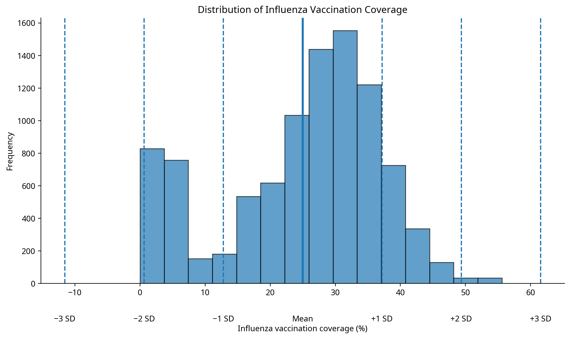

We see that the mean influenza vaccine coverage in the US for those aged 18-49 is 25%. Then, whats the measurement scale? where should we draw the ticks on our ruler? One idea is to use every std (or say a 1/2 standard deviation). They are natural to the collected observations and have an interpretastion for alot (2 standard deviations) or a little (0.01 standard deviations). Note the standard deviation for the vaccine coverage is 12%.

Homework¶

XXX
XXX
XXX
XXX
XXX