Time series forecasting applied to infectious diseases#
Traditional data collection assumes that when we collect a series of data points \(d_{1},d_{2},\cdots,d_{n}\) that these data points are independent from one another. In other words, we assume that collecting the data point \(d_{i}\) does not have an impact on the data points generated after \(d_{i+1},d_{i+2},\cdots\).
Time series data assumes that information we collect over time is related. That is, we assume that the data points collected at time \(t\) impacts the data points collected at times \(t+1, t+2, \cdots\).
Statistical language (The “where is the bathroom?” tutorial).#
All of statistics is based on the experiment and modern statistics is based on the random variable.
An experiment is any pheonema that generates an observation from a set of possible outcomes. For example, an experiment can be defined as a human who sits at the nearest intersection records the number of red cars that pass per hours. A more direct experiment could be considered, we observe a series of epidemic weeks and record the number of patients how walk into a healthcare facility as well as the number of those indiviuals who are diagnosed with influenza-like illness (ILI). Here, the experment is alowing one week to pass and the observations per week are (the number of individuals who enter a healthcare facility in the state, the number of individuals diagnosed with ILI).
A random variable, typically defined with capital letters (like \(X,Y,Z\)), maps all possible outcomes form an experiment to a number. For example, we can define the random variable \(X\) to map the number of red cars observed at the intersection to the same integer on the number line. The random variables \(Y\) and \(Z\) can map the number of individuals who attend a health care facility and number diagnosed with ILI to their respective integers. Random variables are very flexible. For example, our experiment may record the type of flu-test administered to an individual. The possible outcomes could be: XXX. We can define a random variable \(T\) that maps X to the value 0, X to the value 1, and all other tests to the value 2.
With a random variable in hand, we can ask probability questions \(P(X=1)\), \(P(X<10)\), \(P(X+Y=5)\) and so on.
Random variables are the building blocks of statistical modeling. They move the experimental process to the numberline where we can use algebra, calculus, etc to manipulate these variables.
RV approach to time series modeling.#
We can define our time series as a single realization of a sequence of random variables. Let the random variables \(X_{1}, X_{2}, \cdots, X_{T}\) represent the set of possible ILI diagnoses at epiweeks 2025W40,2025W41,2025W42, etc. Then, our observed time series data \((x_{1},x_{2},x_{3},\cdots,x_{T})\) is a single realization from these \(T\) random variables. In essence, we played the following game: at time 1 we asked \(X_{1}\) to generate a single observation from all possible ones it could generated. Then we moved to \(X_{2}\) and asked the same question. The replies were stacked in sequence.
The dataset#
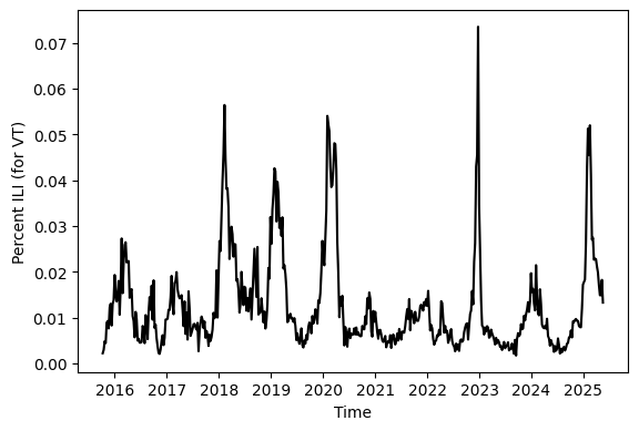
The dataset we will use for lecture is called U.S. Outpatient Influenza-like Illness Surveillance Network, or ILINet. Collection for this dataset began during the 1997/98 season. Data is available via ILINet at the national level, for all 10 health and human services (HHS) regions, as well at state level. ILINet provides the number of patients recorded at outpatient healthcare facilties and the number of those individuals who were diagnosed with influenza-like Illness weekly. For our work here we will study the percent ILI which is defined as the number of those diagnosed with ILI divided by the number of individuals who were recorded at a healthcare facility.
#--import python packages
import pandas as pd
from epiweeks import Week
import matplotlib.pyplot as plt

#--Delphi-Epidata API for collecting ILI data easy
from delphi_epidata import Epidata

ili_data_request_object = Epidata.fluview(regions=['vt'], epiweeks=['201540-202520'])
ili_data                = pd.DataFrame(ili_data_request_object['epidata'])

#--Adding some extra to the ILI dataset
#--i want to add the end date to each MMWR week to help with plot presentation
ili_data["end_date"] = [ Week.fromstring(str(x)).enddate()  for x in ili_data.epiweek.values]
ili_data["ili_prop"] = ili_data.num_ili / ili_data.num_patients

#--plotting our time series data
fig, ax = plt.subplots()
ax.plot( ili_data["end_date"], ili_data["ili_prop"], color = "black" )
ax.set_xlabel("Time")
ax.set_ylabel("Percent ILI (for VT)")
fig.subplots_adjust(bottom=0.20)
plt.show()
The goal for exploratory data analysis (EDA) are to: (1) visualize, or otherwise extract, any characteristic patterns from your time series, (2) detect anamloies or other unusual information in your time series data, (3) test classic assumptions for many time series models, and (4) build a reasonable model.
We will use techniques in EDA to inform how to build a time series model for ILI.
An important forecasting template.#
Before more serious time series models, it is important to briefly explore the random walk. The random walk can teach us a valuable lesson on what we expect to happen to our forecasts intuitively.
A random walk is defined as a sequence of random variables that have a Normal distribution (the bell curve) with the same expected value (mean) of zero and the same standard deviation of \(\sigma\) (pronounced “sigma”) such that
For a random walk, what do we expect to happen to the standard deviation as we progress through time? To gain intuition, we can simulate several random walks for \(T\) time steps.
Any time you wish to use a simulation to build intuition, do the following:
Code one instance
Package this instance and then run many times
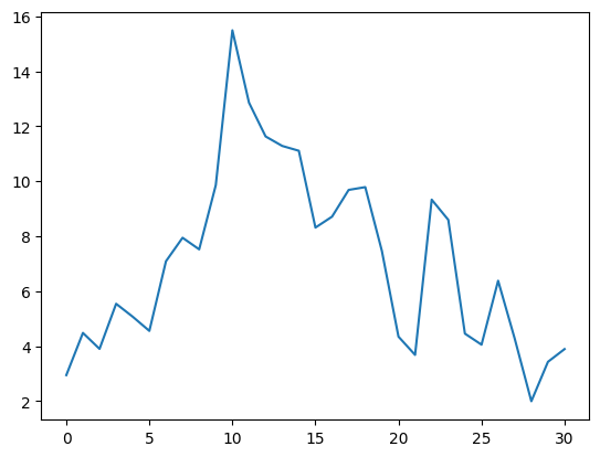
Code one instance#
import numpy as np

standard_deviation = 2.
T                  = 30

z = [np.random.normal(0,standard_deviation)]
for t in range(T):
    N           = np.random.normal(0,standard_deviation)
    z_t_minus_1 = z[-1]
    zt = z_t_minus_1 + N
    z.append(zt)
plt.plot(z)
[<matplotlib.lines.Line2D at 0x7eff8064e650>]
Packages and run many times to gain intuition#
import numpy as np

standard_deviation = 2.
T                  = 30

def generate_random_walk(center=0,standard_deviation=None,T=0):
    z = [np.random.normal(center,standard_deviation)]
    for t in range(T):
        N           = np.random.normal(0,standard_deviation)
        z_t_minus_1 = z[-1]
        zt = z_t_minus_1 + N
        z.append(zt)
    return z

for sim in range(1000):
    random_walk = generate_random_walk(0, standard_deviation, T)
    plt.plot(random_walk, color="blue",alpha=0.15)
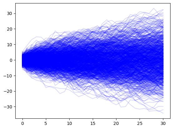
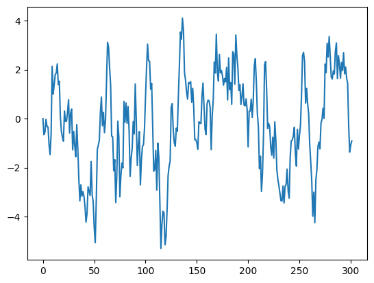
Inuitively, we are less certain as the future progresses.#
As time progresses, the random walk spreads out slowly. This matches with out intuition when building a forecast. We expect that as time progresses away from our observed data, that the uncertainity in our should also grow. Lets look at how to apply a random walk to our ILI data. Though this is a simplistic model, we will extract useful information about how we expect time series models to behave.
Fitting the random walk model to data#
Give a sequence of observations over time \(x_{1},x_{2},x_{3},\cdots,x_{T}\), the random walk supposes that
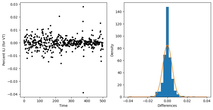
This then means that we expect the differences between two consecutive values to follow a Normal distribution.
For the random walk model, we have a single parameter to estimate: the standard deviation of the size of the difference between two consecutive values. The standard deviation can be computed in all modern software.
Lets plot the difference in the proportion of ILI over time. We’ll look at the raw differneces as well as a histogram.
#--first we compute the differences
differences           = np.diff(ili_data["ili_prop"])
number_of_differences = len(differences)

#--setup a figure and axis to plot our data
fig, axs = plt.subplots(1,2, figsize=(10,5))

##--Take the first axis for plotting a scatter of differences
ax=axs[0]
ax.scatter(np.arange(number_of_differences)
           , differences
           , color = "black"
           , s     = 10)
ax.set_xlabel("Time")
ax.set_ylabel("Percent ILI (for VT)")

##--Take the second axis for plotting a histogram of differences
ax=axs[1]
ax.hist(x=differences,bins=25,density=True)

ax.set_xlabel("Differences")
ax.set_ylabel("Density")

#--Fit a normal curve with zero mean and estimated standard deviation
import scipy.stats
estimated_std = np.std(differences)

domain = np.linspace(-0.04,0.04)
pdf_values = scipy.stats.norm(0,estimated_std).pdf(domain )

plt.plot(domain, pdf_values)

plt.show()
Forecasting with a random walk#
Note that our specification for the random walk was
but we didnt specify for what time units this model holds. Even more, we didnt specify how we will use this model to build a forecast.
A forecast is a sequence of probability distributions—often represented by random variables—over a sequence of future time units. Lets spend time better specifying our random walk model
for times \(1,2,\cdots T\) where \(T\) is the last observation from our time series data. We will generate a forecast for time units \(T+1\) and so on as
Our random walk model generates a forecast at time \(T+k\) by selecting the last observed value \(x_{T}\) and adding \(k\) draws from a Normal distribution centered at zero with standard deviation \(\sigma^{2}\).
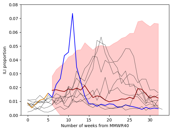
Lets look at VT ILI data again and fit a random walk model. We will assume that we have observed the first 6 weeks (MMWRWK40-MMWRWK46) of the 2022/2023 season. We will estimate the standard deviation of our differences (ie fitting the model) and we will generate a 5 week ahead forecast.
#--Aside: this adds season data to our ILI dataset
def add_season(row):
    from epiweeks import Week
    epiweek = str(row.epiweek)
    yr = int(epiweek[:4])
    wk = int(epiweek[-2:])

    w = Week(yr,wk)

    if w.week >=40:
        return "{:02d}/{:02d}".format( yr,yr+1 )
    elif w.week <=20:
        return "{:02d}/{:02d}".format( yr-1,yr )
    else:
        return "offseason"
ili_data["season"] = [ add_season(row) for i,row in ili_data.iterrows()]

#--remove the offseason for our analysis
ili_data = ili_data.loc[ ili_data.season!="offseason" ]

#--Lets select the 2022/2023 datset
one_season = ili_data.loc[ ili_data.season == "2022/2023" ]

#--extract the ILI proportion values
one_season_ili = one_season.ili_prop.values

#--assume that we only have information up to MMWRWK46
one_season_hidden = one_season_ili[:6]

#--visualize
fig,ax = plt.subplots()

#--plot the whole ILI curve
ax.plot(one_season_ili, color = "blue", label = "2022/2023")

#--plot the observed curve up to MMWR46
ax.plot(one_season_hidden, label = "observed", color="orange")

#--Estimate the standard deviation of the differences (ie fit the model)
differences                  = np.diff(one_season_hidden)
estimated_standard_deviation = np.std(differences)

#--Generate our forecast
last_value = one_season_hidden[-1]
for sim in range(1000):
    rw = generate_random_walk(center = last_value, standard_deviation=estimated_standard_deviation, T=5)

    #--This is how you label just one curve for your legend
    ax.plot( np.arange(5,6+5+1), [last_value] + list(rw),color="red",alpha=0.05)

#--labels
ax.set_xlabel("Number of weeks from MMWR40")
ax.set_ylabel("ILI proportion")

ax.set_ylim(0,0.08)

#--add legend and show plot
ax.legend()
plt.show()
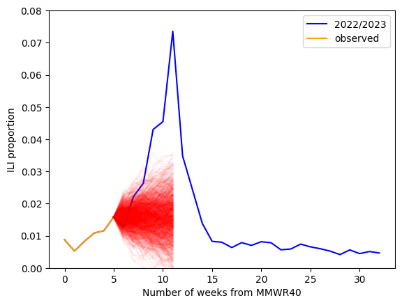
What can we learn from studying, and then fitting by hand, the random walk model? The uncertainity in the random walk, and in many time series models, is characterized by the standard deviation. So, we expect that for most time series models the standard deviation should depend on properties of our model (ie the random walk), how much data we collected (to better estimate our standard deviation), and, importantly, should depend on time.
In addition, we should be careful to specify how we fit our model to observed data and how we communicate to others the method we use to generate our forecasts.
AR(1): O, ive seen that in the past! Modeling a single time series.#
Autocorrelation#
A time series dataset is called auto-correlated if there exists a signficant correlation between: (1) subsequent values or (2) values at a regular interval. If a time series doesnt have any auto correlation for any regular time interval than this is a warning that your data may not be best modeled using time-series techniques. Without any auto-corrlelation, subsequent values are unlikely related to those values collected in the past. This will violate the assumptions more most if not all, time series models.
How do we think of auto-correaltion using random variables? Let \(X_{1},X_{2},\cdots,X_{T}\) represent the sequence of random variables that generated our time series. Then we may observe that values at one time point \(x_{t}\) are not so different from the following value \(x_{t+1}\). This would imply that the random variables \(X_{t}\) and \(X_{t+1}\) are not statistically independent from one another.
To understand the correlation between subsequent values, we can plot \(x_{t+1}\) on the vertical axis and \(x_{t}\) on the horizontal axis. This is often called a lag 1-plot.
fig, ax = plt.subplots()

ili_prop = ili_data.ili_prop.values
ili_prop_at_tp1 = ili_prop[1:]
ili_prop_at_t   = ili_prop[:-1]

ax.scatter( ili_prop_at_t, ili_prop_at_tp1, alpha=0.80, edgecolors="black", facecolors="none")
ax.set_xlabel("ILI at time t")
ax.set_ylabel("ILI at time t+1")

plt.show()
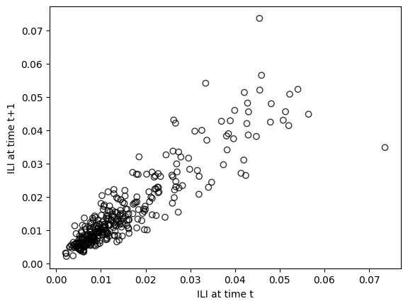
We can see a very pronounced linear trend between ILI at time t and ILI and time t+1. We can quantify that correlation by computing the linear correlation coefficient.
import numpy as np
LCC = np.corrcoef(ili_prop_at_t,ili_prop_at_tp1)[0,1]
print("Linear correlation for Lag 1 = {:.2f}".format(LCC))
Linear correlation for Lag 1 = 0.90
The Auto-regressive model: leveraging the lag-1 plot#
Given a sequence of observations \((x_{1},x_{2},x_{3},\cdots,x_{T})\) from a time-series, an auto-regressive one process [nicknamed AR(1)] assumes that the expected value at time \(t+1\) has a linear relationship that depends on the observed value in the time series at time \(t\). This linear relationship between the expected value at time \(t+1\) and previously observed value cane be written mathematically as
where the symbol \(\mathbb{E}\) is called the expected value. The AR1 model also assumes a Normal distribution that is centered around this expected value \( \mathbb{E}(x_{t+1})\).
Note
The Normal distribution is a distribution of non-surprisal, data close to the mean, or expectitude. The probability that we would find a value outside of two standard deviations from the expected value for a normal distribution is less than 5%. When a statistican or similar uses a Normal distribution with mean \(\mu\) then you should think “ok, the statistician is communicating to me that the value is basically \(\mu\)”
The first way to write down the AR1 model is
This says (1) i think that the distribution of values at \(x_{t+1}\) looks like a bell-curve (Normal) (2) i think that this next value is quite close to \(\beta_{0}+\beta_{1}x_t\), and (3) i think that this next value depends on \(x_{t}\). An alternative way to write down this model focuses more on the expected value,
Fitting the model#
from statsmodels.tsa.ar_model import AutoReg
model = AutoReg(ili_data.ili_prop.values, 1).fit()
print(model.summary())
                            AutoReg Model Results
==============================================================================
Dep. Variable:                      y   No. Observations:                  331
Model:                     AutoReg(1)   Log Likelihood                1273.540
Method:               Conditional MLE   S.D. of innovations              0.005
Date:                Thu, 16 Oct 2025   AIC                          -2541.081
Time:                        03:54:49   BIC                          -2529.683
Sample:                             1   HQIC                         -2536.534
                                  331
==============================================================================
                 coef    std err          z      P>|z|      [0.025      0.975]
------------------------------------------------------------------------------
const          0.0016      0.000      3.442      0.001       0.001       0.003
y.L1           0.8990      0.024     37.672      0.000       0.852       0.946
                                    Roots
=============================================================================
                  Real          Imaginary           Modulus         Frequency
-----------------------------------------------------------------------------
AR.1            1.1123           +0.0000j            1.1123            0.0000
-----------------------------------------------------------------------------
#--extract the ILI proportion values
one_season_ili = one_season.ili_prop.values

#--assume that we only have information up to MMWRWK46
one_season_hidden = one_season_ili[:6]

weeks = np.arange(len(one_season_hidden))

from statsmodels.tsa.ar_model import AutoReg
model = AutoReg(one_season_hidden, 1).fit()
print(model.summary())


h=5
pred    = model.get_prediction(start= 6, end=6+h)
fc_mean = pred.predicted_mean
fc_ci   = pred.conf_int(alpha=0.20)

fig,ax = plt.subplots()

ax.plot(one_season_ili, color = "blue", label = "2022/2023" )
ax.plot( weeks, one_season_hidden , color = "orange", label = "Observed" )

ax.plot( 5+np.arange(len(one_season_hidden)+1), [one_season_hidden[-1]]+list(fc_mean), color ="darkred")
ax.fill_between( 5+np.arange(len(one_season_hidden)+1)
                 , [one_season_hidden[-1]] + list(fc_ci[:,0])
                 , [one_season_hidden[-1]] + list(fc_ci[:,1])
                 , alpha=0.50, color="red")

ax.set_xlabel("Number of weeks from MMWR40")
ax.set_ylabel("ILI proportion")

ax.set_ylim(0,0.08)

differences                  = np.diff(one_season_hidden)
estimated_standard_deviation = np.std(differences)

rw_samples = []
for sim in range(1000):
    rw = generate_random_walk(center = last_value, standard_deviation=estimated_standard_deviation, T=5)
    rw_samples.append([last_value] + list(rw))
rw_samples = np.array(rw_samples)

lower_10,median,upper_90 = np.percentile(rw_samples, [10,50,90],axis=0)

#--This is how you label just one curve for your legend
ax.plot( np.arange(5,6+5+1), median ,color="purple",alpha=1)
ax.fill_between( np.arange(5,6+5+1), lower_10, upper_90 ,color="purple",alpha=0.25)

#--add legend and show plot
ax.legend()
plt.show()
                            AutoReg Model Results
==============================================================================
Dep. Variable:                      y   No. Observations:                    6
Model:                     AutoReg(1)   Log Likelihood                  22.454
Method:               Conditional MLE   S.D. of innovations              0.003
Date:                Thu, 16 Oct 2025   AIC                            -38.908
Time:                        03:54:49   BIC                            -40.080
Sample:                             1   HQIC                           -42.053
                                    6
==============================================================================
                 coef    std err          z      P>|z|      [0.025      0.975]
------------------------------------------------------------------------------
const          0.0013      0.005      0.251      0.802      -0.009       0.011
y.L1           1.0170      0.545      1.866      0.062      -0.051       2.086
                                    Roots
=============================================================================
                  Real          Imaginary           Modulus         Frequency
-----------------------------------------------------------------------------
AR.1            0.9832           +0.0000j            0.9832            0.0000
-----------------------------------------------------------------------------
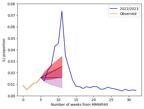
We see that our auto regression (AR) model (in red) better captures the trend in our ILI data compared to a random walk model (in purple). This is especially evident when we compare the forecasts from a random walk and auto regression model. This is because the AR model is able to capture an upward trend in the ILI dataset. The random walk assumes no trend when building a forecast.
Seasonality#
Another noticeable feature of our ILI time series is the repeated pattern of values that all of us have likely observed personally. In statistical literature this is called `seasonality’. A time series is “seasonal” at time interval \(V\) if there exists a correlation between values spaced \(V\) units apart.
We can gain an understanding of seasonality, and correlations at all time intervals, by building an auto-correlation plot. An auto correlation plot is produced by repeating the following two steps.
For time interval \(V\)
Assign the variable \(D_1\) the dataset (x_{1},x_{2},\cdots,x_{T-v}) and the variable \(D_{2}\) the dataset (x_{v},x_{v+1},\cdots,x_{T})
Compute the linear correlation coefficient and call it corr
Plot the point (V,corr)
import statsmodels
from statsmodels.graphics.tsaplots import plot_acf

fig,axs = plt.subplots(1,2, figsize=(12,3))
ax      = axs[0]
ax.plot(ili_data["ili_prop"].values, color = "black" )
ax.set_xlabel("Time")
ax.set_ylabel("Percent ILI (for VT)")

markers = 17+np.arange(0,len(ili_data),34)
ax.vlines(x=markers
          ,ymin=[0]*len(markers)
          ,ymax = [0.07]*len(markers)
          , lw=1
          , color="red")

ax=axs[1]
plot_acf(ili_data.ili_prop.values, lags = 53,ax=ax)
ax.set_xlabel("Lag")
ax.set_ylabel("Linear correlation")

plt.show()
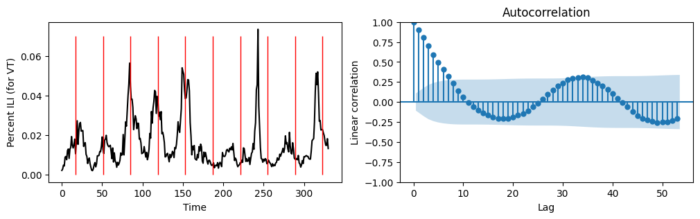
From the above, it looks as though our ILI time series has a strong seasonal pattern. After we remove the “off season” (MMWR weeks 21 to 39), there appear to be a repeating pattern every 34 weeks. This can be confirmed visually (above plot on the left) and can also be confirmed by observing a moderate correlation at a lag of 34 weeks.
Writing down a seasonal AR model#
As a reminder, our non-seasonal AR model looked like this (excluding the intercept for simplicity)
For a seasonal period of \(\ell\), a model with a non-seasonal, lag one autoregressive term plus a seasonal (with period \(\ell\)) lag one autoregressive term looks like this
That is, we expect the ILI value at time \(t+1\) to be related to the previous ILI value one week ago \((x_{t})\) as well as that previous value that appeared last season \(x_{t-\ell}\).
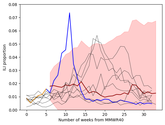
Lets explore fitting a SARIMA model (Seasonal, AutoRegressive, Integrated, Moving Average) to our ILI data. We will fit the model on seasons 2015/16 up until, but no including all of the season 2022/23 data—only the first 6 weeks.
# Assuming 'data' is your time series with a datetime index
# Example for monthly data with a yearly seasonality (m=12)

previous_seasons = []
for year in np.arange(2015,2021+1):
    previous_seasons.append( "{:d}/{:d}".format(year,year+1) )
prev_ili_data = ili_data.loc[ ili_data.season.isin(previous_seasons)  ]
prev_ili = prev_ili_data.ili_prop.values

#--add in the first six observations from the 2022/23 ILI season
all_ili_values = list(prev_ili) + list(one_season_hidden)

import statsmodels.api as sm
model = sm.tsa.SARIMAX( all_ili_values   ,
                       order=(0, 1, 0),
                       seasonal_order=(0, 1, 0, 34))
results = model.fit()
print(results.summary())
                                     SARIMAX Results
==========================================================================================
Dep. Variable:                                  y   No. Observations:                  238
Model:             SARIMAX(0, 1, 0)x(0, 1, 0, 34)   Log Likelihood                 740.324
Date:                            Thu, 16 Oct 2025   AIC                          -1478.648
Time:                                    03:54:50   BIC                          -1475.335
Sample:                                         0   HQIC                         -1477.308
                                            - 238
Covariance Type:                              opg
==============================================================================
                 coef    std err          z      P>|z|      [0.025      0.975]
------------------------------------------------------------------------------
sigma2      3.973e-05   2.91e-06     13.639      0.000     3.4e-05    4.54e-05
===================================================================================
Ljung-Box (L1) (Q):                   7.55   Jarque-Bera (JB):                23.29
Prob(Q):                              0.01   Prob(JB):                         0.00
Heteroskedasticity (H):               1.11   Skew:                            -0.07
Prob(H) (two-sided):                  0.66   Kurtosis:                         4.65
===================================================================================

Warnings:
[1] Covariance matrix calculated using the outer product of gradients (complex-step).
forecast_steps = 32+1-6
pred = results.get_forecast(steps=forecast_steps)          # out-of-sample only
mean_fcst = pred.predicted_mean

ci = pred.conf_int(alpha=0.10)
ci = np.clip(ci,0,np.inf) #<--make sure that these values cannot go below 0

fig,ax = plt.subplots()

ax.plot(one_season_ili, color = "blue", label = "2022/2023" )
ax.plot( weeks, one_season_hidden , color = "orange", label = "Observed" )

ax.plot(6+np.arange(forecast_steps), mean_fcst, color = "darkred")
ax.fill_between(6+np.arange(forecast_steps), ci[:,0],ci[:,1], color = "red", alpha=0.2 )

for season, subset in ili_data.groupby("season"):
    if season in previous_seasons:
        ax.plot( subset.ili_prop.values, color="0.05", lw=0.5  )

#--labels
ax.set_xlabel("Number of weeks from MMWR40")
ax.set_ylabel("ILI proportion")

ax.set_ylim(0,0.08)

plt.show()
MA and differencing#
There is a wide range of different models that we can begin to address with an understanding of the random walk, AR1 model, and the seasonal AR model. But, we should explore two other important concepts in time series forecasting: (1) MA models and (2) differencing.
A moving average (MA) model supposes that future values depend on past model errors. The simplest MA model is the MA(1) model and can be written as
where the error terms \(\epsilon\) all have the same Normal ditribution, \(\mathcal{N}(0,\sigma^{2})\). The difficulty with understanding this model is that if we have not yet observed the \(x\) value at time \(t+1\) when we cannot compute the error \(\epsilon_{t+1}\). This is because
To put it another way, the true errors in our model are never observed.
Lets look at the steps for how we would simulate a MA(1) process to gain intuition for this model. The zeroth and the first x values are
It is typicaly to set \(\epsilon_{-1}\) and \(\epsilon_{0}\) equal to zero. Then \(x_{0}=0\) and \(x_{1} = \)\epsilon_{1} + \theta x_{0}$.
x0      = 0   #<- initial value
std_dev = 1   #<-standard deviation for our error terms
T       = 300 #<- number of time units to simulate
theta   = 0.9 #<- parameter for our MA(1) model

xs = [x0,np.random.normal(0,std_dev)]     #<--start at x0
for time in range(T):
    err = np.random.normal(0,std_dev) #<--draw an error term from N(0,std_dev)
    xs.append( err + theta*xs[-1]  ) #<--propogate time series forward.
plt.plot(xs)
[<matplotlib.lines.Line2D at 0x7eff664c0fd0>]
x0      = 0   #<- initial value
std_dev = 1   #<-standard deviation for our error terms
T       = 300 #<- number of time units to simulate


fig,axs = plt.subplots(1,2,figsize=(10,4))

ax = axs[0]
theta   = 0.1 #<- parameter for our MA(1) model

xs = [x0,np.random.normal(0,std_dev)]     #<--start at x0
for time in range(T):
    err = np.random.normal(0,std_dev) #<--draw an error term from N(0,std_dev)
    xs.append( err + theta*xs[-1]  ) #<--propogate time series forward.
ax.plot(xs)
ax.text(0.95,0.95,s=f"theta = {theta}",ha="right",va="top",transform=ax.transAxes)

ax = axs[1]
theta   = 0.9 #<- parameter for our MA(1) model

xs = [x0,np.random.normal(0,std_dev)]     #<--start at x0
for time in range(T):
    err = np.random.normal(0,std_dev) #<--draw an error term from N(0,std_dev)
    xs.append( err + theta*xs[-1]  ) #<--propogate time series forward.
ax.plot(xs)
ax.text(0.95,0.95,s=f"theta = {theta}",ha="right",va="top",transform=ax.transAxes)

plt.show()
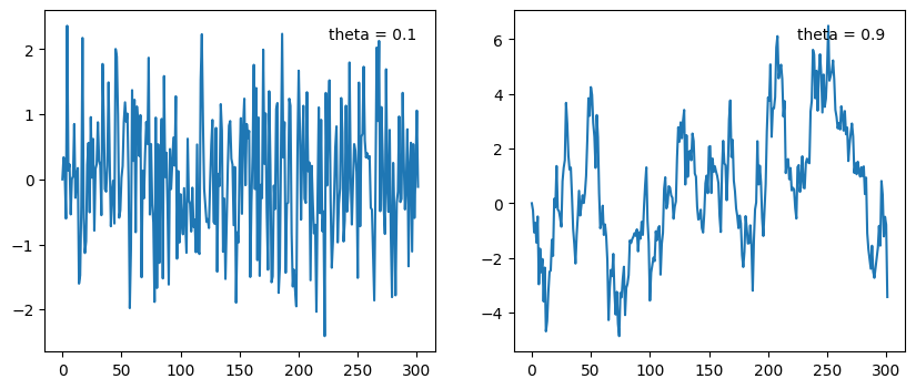
Moving average models are good when random errors (often called shocks) to a system should be (1) propogated over time and (2) errors/shocks further in the past should have a smaller impact on the future when compared to recent shocks to the time series. Theta values close to one carry forward shocks to the system for a long time. Theta values close to zero quickly “forget” shocks to the system. This remember/forget quality can be though of as what length of time should be correlated in the time series.
Differencing#
The AR, MA, and the seasonal variations to these models assume there is no long-term trend in the dataset. If this occurs then a common approach for “detrending” the dataset is to difference it. A one lag difference in a time series model assumes
This might look familar if we rewrite it.
This is the random walk model that we discussed at the very beginning of this class session. In many cases, a first difference removes trend and is amenable to AR, MA types of models. For the sake of detail, a second difference takes the difference of a sequence of time series observations that have themselves already been differenced.
If our first-differences time series is
then a second difference is
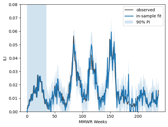
In the model we fit to our ILI dataset, we differenced the ILI values once on a non-seasonal time scale and also once on a seasonal time scale. That is
# Assuming 'data' is your time series with a datetime index
# Example for monthly data with a yearly seasonality (m=12)

previous_seasons = []
for year in np.arange(2015,2021+1):
    previous_seasons.append( "{:d}/{:d}".format(year,year+1) )
prev_ili_data = ili_data.loc[ ili_data.season.isin(previous_seasons)  ]
prev_ili = prev_ili_data.ili_prop.values

#--add in the first six observations from the 2022/23 ILI season
all_ili_values = list(prev_ili) + list(one_season_hidden)

import statsmodels.api as sm
model = sm.tsa.SARIMAX( all_ili_values   ,
                       order=(0, 1, 0),
                       seasonal_order=(0, 1, 0, 34))
results = model.fit()
print(results.summary())

pred_in = results.get_prediction(start=0, end=len(all_ili_values)-1, dynamic=False)
mean_in = pred_in.predicted_mean
ci_in   = pred_in.conf_int(alpha=0.10)   # 90% PI for in-sample one-step-ahead

fig, ax = plt.subplots()
ax.plot(all_ili_values, label="observed", color="0.2")
ax.plot(mean_in, label="in-sample fit", lw=2)

ax.fill_between( np.arange(len(mean_in)), ci_in[:,0], ci_in[:,1], alpha=0.2, label="90% PI")

ax.set_ylim(0,0.08)

ax.legend()
ax.set_xlabel("MMWR Weeks")
ax.set_ylabel("ILI")
plt.show()
                                     SARIMAX Results
==========================================================================================
Dep. Variable:                                  y   No. Observations:                  238
Model:             SARIMAX(0, 1, 0)x(0, 1, 0, 34)   Log Likelihood                 740.324
Date:                            Thu, 16 Oct 2025   AIC                          -1478.648
Time:                                    03:54:51   BIC                          -1475.335
Sample:                                         0   HQIC                         -1477.308
                                            - 238
Covariance Type:                              opg
==============================================================================
                 coef    std err          z      P>|z|      [0.025      0.975]
------------------------------------------------------------------------------
sigma2      3.973e-05   2.91e-06     13.639      0.000     3.4e-05    4.54e-05
===================================================================================
Ljung-Box (L1) (Q):                   7.55   Jarque-Bera (JB):                23.29
Prob(Q):                              0.01   Prob(JB):                         0.00
Heteroskedasticity (H):               1.11   Skew:                            -0.07
Prob(H) (two-sided):                  0.66   Kurtosis:                         4.65
===================================================================================

Warnings:
[1] Covariance matrix calculated using the outer product of gradients (complex-step).
forecast_steps = 34-6
pred = results.get_forecast(steps=forecast_steps)          # out-of-sample only
mean_fcst = pred.predicted_mean

ci = pred.conf_int(alpha=0.10)
ci = np.clip(ci,0,np.inf) #<--make sure that these values cannot go below 0

fig,ax = plt.subplots()

ax.plot(one_season_ili, color = "blue", label = "2022/2023" )
ax.plot( weeks, one_season_hidden , color = "orange", label = "Observed" )

ax.plot(6+np.arange(forecast_steps), mean_fcst, color = "darkred")
ax.fill_between(6+np.arange(forecast_steps), ci[:,0],ci[:,1], color = "red", alpha=0.2 )

for season, subset in ili_data.groupby("season"):
    if season in previous_seasons:
        plt.plot( subset.ili_prop.values, color="0.05", lw=0.5  )

#--labels
ax.set_xlabel("Number of weeks from MMWR40")
ax.set_ylabel("ILI proportion")

ax.set_ylim(0,0.08)
(0.0, 0.08)
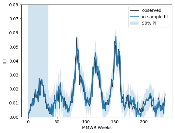
# Assuming 'data' is your time series with a datetime index
# Example for monthly data with a yearly seasonality (m=12)

previous_seasons = []
for year in np.arange(2015,2021+1):
    previous_seasons.append( "{:d}/{:d}".format(year,year+1) )
prev_ili_data = ili_data.loc[ ili_data.season.isin(previous_seasons)  ]
prev_ili = prev_ili_data.ili_prop.values

#--add in the first six observations from the 2022/23 ILI season
all_ili_values = list(prev_ili) + list(one_season_hidden)

import statsmodels.api as sm
model = sm.tsa.SARIMAX( all_ili_values   ,
                       order=(0, 1, 1),
                       seasonal_order=(0, 1, 1, 34))
results = model.fit()
print(results.summary())

pred_in = results.get_prediction(start=0, end=len(all_ili_values)-1, dynamic=False)
mean_in = pred_in.predicted_mean
ci_in   = pred_in.conf_int(alpha=0.10)   # 90% PI for in-sample one-step-ahead

fig, ax = plt.subplots()
ax.plot(all_ili_values, label="observed", color="0.2")
ax.plot(mean_in, label="in-sample fit", lw=2)

ax.fill_between( np.arange(len(mean_in)), ci_in[:,0], ci_in[:,1], alpha=0.2, label="90% PI")

ax.set_ylim(0,0.08)

ax.legend()
ax.set_xlabel("MMWR Weeks")
ax.set_ylabel("ILI")
plt.show()
                                     SARIMAX Results
==========================================================================================
Dep. Variable:                                  y   No. Observations:                  238
Model:             SARIMAX(0, 1, 1)x(0, 1, 1, 34)   Log Likelihood                 781.851
Date:                            Thu, 16 Oct 2025   AIC                          -1557.702
Time:                                    03:54:57   BIC                          -1547.762
Sample:                                         0   HQIC                         -1553.681
                                            - 238
Covariance Type:                              opg
==============================================================================
                 coef    std err          z      P>|z|      [0.025      0.975]
------------------------------------------------------------------------------
ma.L1         -0.1086      0.072     -1.501      0.133      -0.250       0.033
ma.S.L34      -0.9346      0.400     -2.338      0.019      -1.718      -0.151
sigma2      2.017e-05   7.24e-06      2.787      0.005    5.99e-06    3.44e-05
===================================================================================
Ljung-Box (L1) (Q):                   0.02   Jarque-Bera (JB):                29.86
Prob(Q):                              0.88   Prob(JB):                         0.00
Heteroskedasticity (H):               0.72   Skew:                            -0.17
Prob(H) (two-sided):                  0.17   Kurtosis:                         4.85
===================================================================================

Warnings:
[1] Covariance matrix calculated using the outer product of gradients (complex-step).
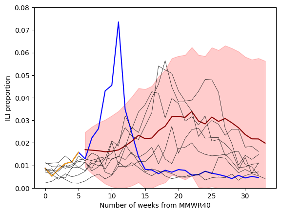
forecast_steps = 34-6
pred = results.get_forecast(steps=forecast_steps)          # out-of-sample only
mean_fcst = pred.predicted_mean

ci = pred.conf_int(alpha=0.10)
ci = np.clip(ci,0,np.inf) #<--make sure that these values cannot go below 0

fig,ax = plt.subplots()

ax.plot(one_season_ili, color = "blue", label = "2022/2023" )
ax.plot( weeks, one_season_hidden , color = "orange", label = "Observed" )

ax.plot(6+np.arange(forecast_steps), mean_fcst, color = "darkred")
ax.fill_between(6+np.arange(forecast_steps), ci[:,0],ci[:,1], color = "red", alpha=0.2 )

for season, subset in ili_data.groupby("season"):
    if season in previous_seasons:
        plt.plot( subset.ili_prop.values, color="0.05", lw=0.5  )

#--labels
ax.set_xlabel("Number of weeks from MMWR40")
ax.set_ylabel("ILI proportion")

ax.set_ylim(0,0.08)
(0.0, 0.08)
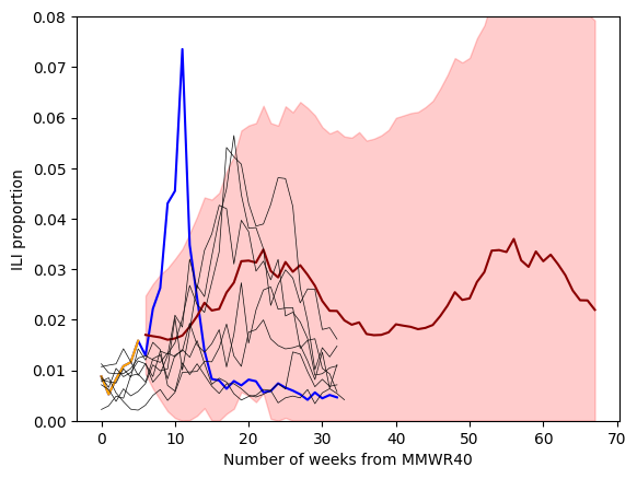
forecast_steps = 2*34-6
pred = results.get_forecast(steps=forecast_steps)          # out-of-sample only
mean_fcst = pred.predicted_mean

ci = pred.conf_int(alpha=0.10)
ci = np.clip(ci,0,np.inf) #<--make sure that these values cannot go below 0

fig,ax = plt.subplots()

ax.plot(one_season_ili, color = "blue", label = "2022/2023" )
ax.plot( weeks, one_season_hidden , color = "orange", label = "Observed" )

ax.plot(6+np.arange(forecast_steps), mean_fcst, color = "darkred")
ax.fill_between(6+np.arange(forecast_steps), ci[:,0],ci[:,1], color = "red", alpha=0.2 )

for season, subset in ili_data.groupby("season"):
    if season in previous_seasons:
        plt.plot( subset.ili_prop.values, color="0.05", lw=0.5  )

#--labels
ax.set_xlabel("Number of weeks from MMWR40")
ax.set_ylabel("ILI proportion")

ax.set_ylim(0,0.08)
(0.0, 0.08)